Pyomo.DoE

Pyomo.DoE (Pyomo Design of Experiments) is a Python library for model-based design of experiments using science-based models.

Pyomo.DoE was developed by Jialu Wang and Alexander W. Dowling at the University of Notre Dame as part of the Carbon Capture Simulation for Industry Impact (CCSI2). project, funded through the U.S. Department Of Energy Office of Fossil Energy.

If you use Pyomo.DoE, please cite:

[Wang and Dowling, 2022] Wang, Jialu, and Alexander W. Dowling. “Pyomo.DOE: An open‐source package for model‐based design of experiments in Python.” AIChE Journal 68.12 (2022): e17813. https://doi.org/10.1002/aic.17813

Methodology Overview

Model-based Design of Experiments (MBDoE) is a technique to maximize the information gain of experiments by directly using science-based models with physically meaningful parameters. It is one key component in the model calibration and uncertainty quantification workflow shown below:

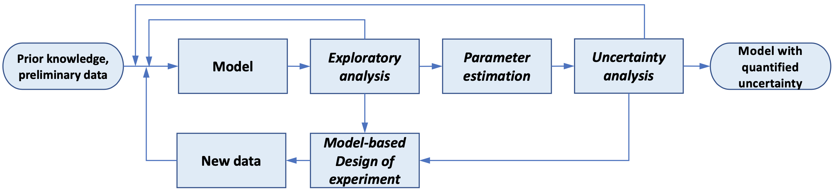
Fig. 2 The exploratory analysis, parameter estimation, uncertainty analysis, and MBDoE are combined into an iterative framework to select, refine, and calibrate science-based mathematical models with quantified uncertainty. Currently, Pyomo.DoE focuses on increasing parameter precision.

Pyomo.DoE provides the exploratory analysis and MBDoE capabilities to the Pyomo ecosystem. The user provides one Pyomo model, a set of parameter nominal values, the allowable design spaces for design variables, and the assumed observation error model. During exploratory analysis, Pyomo.DoE checks if the model parameters can be inferred from the postulated measurements or preliminary data. MBDoE then recommends optimized experimental conditions for collecting more data. Parameter estimation packages such as Parmest can perform parameter estimation using the available data to infer values for parameters, and facilitate an uncertainty analysis to approximate the parameter covariance matrix. If the parameter uncertainties are sufficiently small, the workflow terminates and returns the final model with quantified parametric uncertainty. If not, MBDoE recommends optimized experimental conditions to generate new data.

Below is an overview of the type of optimization models Pyomo.DoE can accommodate:

• Pyomo.DoE is suitable for optimization models of continuous variables

• Pyomo.DoE can handle equality constraints defining state variables

• Pyomo.DoE supports (Partial) Differential-Algebraic Equations (PDAE) models via Pyomo.DAE

• Pyomo.DoE also supports models with only algebraic constraints

The general form of a DAE problem that can be passed into Pyomo.DoE is shown below:

\[\begin{split}\begin{align*} & \dot{\mathbf{x}}(t) = \mathbf{f}(\mathbf{x}(t), \mathbf{z}(t), \mathbf{y}(t), \mathbf{u}(t), \overline{\mathbf{w}}, \boldsymbol{\theta}) \\ & \mathbf{g}(\mathbf{x}(t), \mathbf{z}(t), \mathbf{y}(t), \mathbf{u}(t), \overline{\mathbf{w}},\boldsymbol{\theta})=\mathbf{0} \\ & \mathbf{y} =\mathbf{h}(\mathbf{x}(t), \mathbf{z}(t), \mathbf{u}(t), \overline{\mathbf{w}},\boldsymbol{\theta}) \\ & \mathbf{f}^{\mathbf{0}}\left(\dot{\mathbf{x}}\left(t_{0}\right), \mathbf{x}\left(t_{0}\right), \mathbf{z}(t_0), \mathbf{y}(t_0), \mathbf{u}\left(t_{0}\right), \overline{\mathbf{w}}, \boldsymbol{\theta})\right)=\mathbf{0} \\ & \mathbf{g}^{\mathbf{0}}\left( \mathbf{x}\left(t_{0}\right),\mathbf{z}(t_0), \mathbf{y}(t_0), \mathbf{u}\left(t_{0}\right), \overline{\mathbf{w}}, \boldsymbol{\theta}\right)=\mathbf{0}\\ &\mathbf{y}^{\mathbf{0}}\left(t_{0}\right)=\mathbf{h}\left(\mathbf{x}\left(t_{0}\right),\mathbf{z}(t_0), \mathbf{u}\left(t_{0}\right), \overline{\mathbf{w}}, \boldsymbol{\theta}\right) \end{align*}\end{split}\]

where:

• \(\boldsymbol{\theta} \in \mathbb{R}^{N_p}\) are unknown model parameters.

• \(\mathbf{x} \subseteq \mathcal{X}\) are dynamic state variables which characterize trajectory of the system, \(\mathcal{X} \in \mathbb{R}^{N_x \times N_t}\).

• \(\mathbf{z} \subseteq \mathcal{Z}\) are algebraic state variables, \(\mathcal{Z} \in \mathbb{R}^{N_z \times N_t}\).

• \(\mathbf{u} \subseteq \mathcal{U}\) are time-varying decision variables, \(\mathcal{U} \in \mathbb{R}^{N_u \times N_t}\).

• \(\overline{\mathbf{w}} \in \mathbb{R}^{N_w}\) are time-invariant decision variables.

• \(\mathbf{y} \subseteq \mathcal{Y}\) are measurement response variables, \(\mathcal{Y} \in \mathbb{R}^{N_r \times N_t}\).

• \(\mathbf{f}(\cdot)\) are differential equations.

• \(\mathbf{g}(\cdot)\) are algebraic equations.

• \(\mathbf{h}(\cdot)\) are measurement functions.

• \(\mathbf{t} \in \mathbb{R}^{N_t \times 1}\) is a union of all time sets.

Note

• Parameters and design variables should be defined as Pyomo Var components on the model to use direct_kaug mode, and can be defined as Pyomo Param object if not using direct_kaug.

Based on the above notation, the form of the MBDoE problem addressed in Pyomo.DoE is shown below:

\[\begin{split}\begin{equation} \begin{aligned} \underset{\boldsymbol{\varphi}}{\max} \quad & \Psi (\mathbf{M}(\mathbf{\hat{y}}, \boldsymbol{\varphi})) \\ \text{s.t.} \quad & \mathbf{M}(\boldsymbol{\hat{\theta}}, \boldsymbol{\varphi}) = \sum_r^{N_r} \sum_{r'}^{N_r} \tilde{\sigma}_{(r,r')}\mathbf{Q}_r^\mathbf{T} \mathbf{Q}_{r'} + \mathbf{V}^{-1}_{\boldsymbol{\theta}}(\boldsymbol{\hat{\theta}}) \\ & \dot{\mathbf{x}}(t) = \mathbf{f}(\mathbf{x}(t), \mathbf{z}(t), \mathbf{y}(t), \mathbf{u}(t), \overline{\mathbf{w}}, \boldsymbol{\theta}) \\ & \mathbf{g}(\mathbf{x}(t), \mathbf{z}(t), \mathbf{y}(t), \mathbf{u}(t), \overline{\mathbf{w}},\boldsymbol{\theta})=\mathbf{0} \\ & \mathbf{y} =\mathbf{h}(\mathbf{x}(t), \mathbf{z}(t), \mathbf{u}(t), \overline{\mathbf{w}},\boldsymbol{\theta}) \\ & \mathbf{f}^{\mathbf{0}}\left(\dot{\mathbf{x}}\left(t_{0}\right), \mathbf{x}\left(t_{0}\right), \mathbf{z}(t_0), \mathbf{y}(t_0), \mathbf{u}\left(t_{0}\right), \overline{\mathbf{w}}, \boldsymbol{\theta})\right)=\mathbf{0} \\ & \mathbf{g}^{\mathbf{0}}\left( \mathbf{x}\left(t_{0}\right),\mathbf{z}(t_0), \mathbf{y}(t_0), \mathbf{u}\left(t_{0}\right), \overline{\mathbf{w}}, \boldsymbol{\theta}\right)=\mathbf{0}\\ &\mathbf{y}^{\mathbf{0}}\left(t_{0}\right)=\mathbf{h}\left(\mathbf{x}\left(t_{0}\right),\mathbf{z}(t_0), \mathbf{u}\left(t_{0}\right), \overline{\mathbf{w}}, \boldsymbol{\theta}\right) \end{aligned} \end{equation}\end{split}\]

where:

• \(\boldsymbol{\varphi}\) are design variables, which are manipulated to maximize the information content of experiments. It should consist of one or more of \(\mathbf{u}(t), \mathbf{y}^{\mathbf{0}}({t_0}),\overline{\mathbf{w}}\). With a proper model formulation, the timepoints for control or measurements \(\mathbf{t}\) can also be degrees of freedom.

• \(\mathbf{M}\) is the Fisher information matrix (FIM), estimated as the inverse of the covariance matrix of parameter estimates \(\boldsymbol{\hat{\theta}}\). A large FIM indicates more information contained in the experiment for parameter estimation.

• \(\mathbf{Q}\) is the dynamic sensitivity matrix, containing the partial derivatives of \(\mathbf{y}\) with respect to \(\boldsymbol{\theta}\).

• \(\Psi\) is the design criteria to measure FIM.

• \(\mathbf{V}_{\boldsymbol{\theta}}(\boldsymbol{\hat{\theta}})^{-1}\) is the FIM of previous experiments.

Pyomo.DoE provides four design criteria \(\Psi\) to measure the size of FIM:

Table 2 Pyomo.DoE design criteria

Design criterion	Computation	Geometrical meaning
A-optimality	\(\text{trace}({\mathbf{M}})\)	Dimensions of the enclosing box of the confidence ellipse
D-optimality	\(\text{det}({\mathbf{M}})\)	Volume of the confidence ellipse
E-optimality	\(\text{min eig}({\mathbf{M}})\)	Size of the longest axis of the confidence ellipse
Modified E-optimality	\(\text{cond}({\mathbf{M}})\)	Ratio of the longest axis to the shortest axis of the confidence ellipse

In order to solve problems of the above, Pyomo.DoE implements the 2-stage stochastic program. Please see Wang and Dowling (2022) for details.

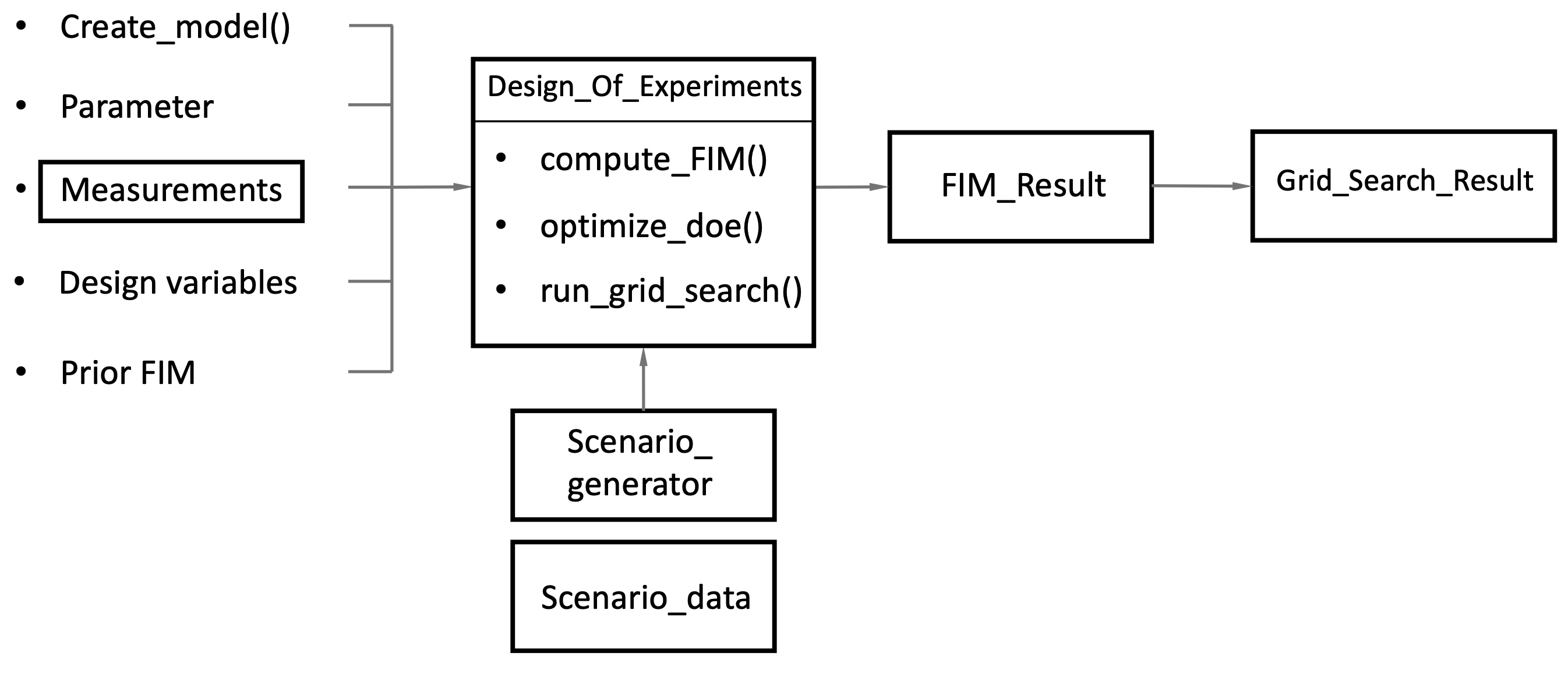
Pyomo.DoE Required Inputs

The required inputs to the Pyomo.DoE solver are the following:

• A function that creates the process model

• Dictionary of parameters and their nominal value

• A measurement object

• A design variables object

• A Numpy array containing the Prior FIM

• Optimization solver

Below is a list of arguments that Pyomo.DoE expects the user to provide.

parameter_dictdictionary

A dictionary of parameter names and values. If they are an indexed variable, put the variable name and index in a nested Dictionary.

design_variables: DesignVariables

A DesignVariables of design variables, provided by the DesignVariables class. If this design var is independent of time (constant), set the time to [0]

measurement_variablesMeasurementVariables

A MeasurementVariables of the measurements, provided by the MeasurementVariables class.

create_modelfunction

A function returning a deterministic process model.

prior_FIMarray

An array defining the Fisher information matrix (FIM) for prior experiments, default is a zero matrix.

Pyomo.DoE Solver Interface

class pyomo.contrib.doe.doe.DesignOfExperiments(param_init, design_vars, measurement_vars, create_model, solver=None, prior_FIM=None, discretize_model=None, args=None)

__init__(param_init, design_vars, measurement_vars, create_model, solver=None, prior_FIM=None, discretize_model=None, args=None)

This package enables model-based design of experiments analysis with Pyomo. Both direct optimization and enumeration modes are supported. NLP sensitivity tools, e.g., sipopt and k_aug, are supported to accelerate analysis via enumeration. It can be applied to dynamic models, where design variables are controlled throughout the experiment.

Parameters:

• param_init – A dictionary of parameter names and values. If they defined as indexed Pyomo variable, put the variable name and index, such as ‘theta[“A1”]’.

• design_vars – A DesignVariables which contains the Pyomo variable names and their corresponding indices and bounds for experiment degrees of freedom

• measurement_vars – A MeasurementVariables which contains the Pyomo variable names and their corresponding indices and bounds for experimental measurements

• create_model – A Python function that returns a Concrete Pyomo model, similar to the interface for parmest

• solver – A solver object that User specified, default=None. If not specified, default solver is IPOPT MA57.

• prior_FIM – A 2D numpy array containing Fisher information matrix (FIM) for prior experiments. The default None means there is no prior information.

• discretize_model – A user-specified function that discretizes the model. Only use with Pyomo.DAE, default=None

• args – Additional arguments for the create_model function.

compute_FIM(mode='direct_kaug', FIM_store_name=None, specified_prior=None, tee_opt=True, scale_nominal_param_value=False, scale_constant_value=1, store_output=None, read_output=None, extract_single_model=None, formula='central', step=0.001)

This function calculates the Fisher information matrix (FIM) using sensitivity information obtained from two possible modes (defined by the CalculationMode Enum):

1. sequential_finite: sequentially solve square problems and use finite difference approximation

2. direct_kaug: solve a single square problem then extract derivatives using NLP sensitivity theory

Parameters:

• mode – supports CalculationMode.sequential_finite or CalculationMode.direct_kaug

• FIM_store_name – if storing the FIM in a .csv or .txt, give the file name here as a string.

• specified_prior – a 2D numpy array providing alternate prior matrix, default is no prior.

• tee_opt – if True, IPOPT console output is printed

• scale_nominal_param_value – if True, the parameters are scaled by its own nominal value in param_init

• scale_constant_value – scale all elements in Jacobian matrix, default is 1.

• store_output – if storing the output (value stored in Var ‘output_record’) as a pickle file, give the file name here as a string.

• read_output – if reading the output (value for Var ‘output_record’) as a pickle file, give the file name here as a string.

• extract_single_model – if True, the solved model outputs for each scenario are all recorded as a .csv file. The output file uses the name AB.csv, where string A is store_output input, B is the index of scenario. scenario index is the number of the scenario outputs which is stored.

• formula – choose from the Enum FiniteDifferenceStep.central, .forward, or .backward. This option is only used for CalculationMode.sequential_finite mode.

• step – Sensitivity perturbation step size, a fraction between [0,1]. default is 0.001

Returns:

FIM_analysis

Return type:

result summary object of this solve

run_grid_search(design_ranges, mode='sequential_finite', tee_option=False, scale_nominal_param_value=False, scale_constant_value=1, store_name=None, read_name=None, store_optimality_as_csv=None, formula='central', step=0.001)

Enumerate through full grid search for any number of design variables; solve square problems sequentially to compute FIMs. It calculates FIM with sensitivity information from two modes:

1. sequential_finite: Calculates a one scenario model multiple times for multiple scenarios. Sensitivity info estimated by finite difference

2. direct_kaug: calculate sensitivity by k_aug with direct sensitivity

Parameters:

• design_ranges – a dict, keys are design variable names, values are a list of design variable values to go over

• mode – choose from CalculationMode.sequential_finite, .direct_kaug.

• tee_option – if solver console output is made

• scale_nominal_param_value – if True, the parameters are scaled by its own nominal value in param_init

• scale_constant_value – scale all elements in Jacobian matrix, default is 1.

• store_name – a string of file name. If not None, store results with this name. It is a pickle file containing all measurement information after solving the model with perturbations. Since there are multiple experiments, results are numbered with a scalar number, and the result for one grid is ‘store_name(count).csv’ (count is the number of count).

• read_name – a string of file name. If not None, read result files. It should be a pickle file previously generated by store_name option. Since there are multiple experiments, this string should be the common part of all files; Real name of the file is “read_name(count)”, where count is the number of the experiment.

• store_optimality_as_csv – if True, the design criterion values of grid search results stored with this file name as a csv

• formula – choose from FiniteDifferenceStep.central, .forward, or .backward. This option is only used for CalculationMode.sequential_finite.

• step – Sensitivity perturbation step size, a fraction between [0,1]. default is 0.001

Returns:

figure_draw_object

Return type:

a combined result object of class Grid_search_result

stochastic_program(if_optimize=True, objective_option='det', scale_nominal_param_value=False, scale_constant_value=1, optimize_opt=None, if_Cholesky=False, L_LB=1e-07, L_initial=None, jac_initial=None, fim_initial=None, formula='central', step=0.001, tee_opt=True)

Optimize DOE problem with design variables being the decisions. The DOE model is formed invasively and all scenarios are computed simultaneously. The function will first run a square problem with design variable being fixed at the given initial points (Objective function being 0), then a square problem with design variables being fixed at the given initial points (Objective function being Design optimality), and then unfix the design variable and do the optimization.

Parameters:

• if_optimize – if true, continue to do optimization. else, just run square problem with given design variable values

• objective_option – choose from the ObjectiveLib enum, “det”: maximizing the determinant with ObjectiveLib.det, “trace”: or the trace of the FIM with ObjectiveLib.trace

• scale_nominal_param_value – if True, the parameters are scaled by its own nominal value in param_init

• scale_constant_value – scale all elements in Jacobian matrix, default is 1.

• optimize_opt – A dictionary, keys are design variables, values are True or False deciding if this design variable will be optimized as DOF or not

• if_Cholesky – if True, Cholesky decomposition is used for Objective function for D-optimality.

• L_LB – L is the Cholesky decomposition matrix for FIM, i.e. FIM = L*L.T. L_LB is the lower bound for every element in L. if FIM is positive definite, the diagonal element should be positive, so we can set a LB like 1E-10

• L_initial – initialize the L

• jac_initial – a matrix used to initialize jacobian matrix

• fim_initial – a matrix used to initialize FIM matrix

• formula – choose from “central”, “forward”, “backward”, which refers to the Enum FiniteDifferenceStep.central, .forward, or .backward

• step – Sensitivity perturbation step size, a fraction between [0,1]. default is 0.001

• tee_opt – if True, IPOPT console output is printed

Returns:

• analysis_square (result summary of the square problem solved at the initial point)

• analysis_optimize (result summary of the optimization problem solved)

Note

stochastic_program() includes the following steps:

1. Build two-stage stochastic programming optimization model where scenarios correspond to finite difference approximations for the Jacobian of the response variables with respect to calibrated model parameters

2. Fix the experiment design decisions and solve a square (i.e., zero degrees of freedom) instance of the two-stage DOE problem. This step is for initialization.

3. Unfix the experiment design decisions and solve the two-stage DOE problem.

class pyomo.contrib.doe.measurements.MeasurementVariables

__init__()

This class stores information on which algebraic and differential variables in the Pyomo model are considered measurements.

add_variables(var_name, indices=None, time_index_position=None, variance=1)

Parameters:

• var_name (a list of var names) –

• indices (a dict containing indices) – if default (None), no extra indices needed for all var in var_name for e.g., {0:[“CA”, “CB”, “CC”], 1: [1,2,3]}.

• time_index_position (an integer indicates which index is the time index) – for e.g., 1 is the time index position in the indices example.

• variance (a scalar number, which is the variance for this measurement.) –

class pyomo.contrib.doe.measurements.DesignVariables

Define design variables

__init__()

This class provides utility methods for DesignVariables and MeasurementVariables to create lists of Pyomo variable names with an arbitrary number of indices.

add_variables(var_name, indices=None, time_index_position=None, values=None, lower_bounds=None, upper_bounds=None)

Parameters:

• var_name (a list of var names) –

• indices (a dict containing indices) – if default (None), no extra indices needed for all var in var_name for e.g., {0:[“CA”, “CB”, “CC”], 1: [1,2,3]}.

• time_index_position (an integer indicates which index is the time index) – for e.g., 1 is the time index position in the indices example.

• values (a list containing values which has the same shape of flattened variables) – default choice is None, means there is no give nvalues

• lower_bounds (a list of lower bounds. If given a scalar number, it is set as the lower bounds for all variables.) –

• upper_bounds (a list of upper bounds. If given a scalar number, it is set as the upper bounds for all variables.) –

class pyomo.contrib.doe.scenario.ScenarioGenerator(parameter_dict=None, formula='central', step=0.001, store=False)

__init__(parameter_dict=None, formula='central', step=0.001, store=False)

Generate scenarios. DoE library first calls this function to generate scenarios.

Parameters:

• parameter_dict – a dict of parameter, keys are names of ‘’string’’, values are their nominal value of ‘’float’’. for e.g., {‘A1’: 84.79, ‘A2’: 371.72, ‘E1’: 7.78, ‘E2’: 15.05}

• formula – choose from ‘central’, ‘forward’, ‘backward’, None.

• step – Sensitivity perturbation step size, a fraction between [0,1]. default is 0.001

• store – if True, store results.

class pyomo.contrib.doe.result.FisherResults(parameter_names, measurements, jacobian_info=None, all_jacobian_info=None, prior_FIM=None, store_FIM=None, scale_constant_value=1, max_condition_number=1000000000000.0)

__init__(parameter_names, measurements, jacobian_info=None, all_jacobian_info=None, prior_FIM=None, store_FIM=None, scale_constant_value=1, max_condition_number=1000000000000.0)

Analyze the FIM result for a single run

Parameters:

• parameter_names – A list of parameter names

• measurements – A MeasurementVariables which contains the Pyomo variable names and their corresponding indices and bounds for experimental measurements

• jacobian_info – the jacobian for this measurement object

• all_jacobian_info – the overall jacobian

• prior_FIM – if there’s prior FIM to be added

• store_FIM – if storing the FIM in a .csv or .txt, give the file name here as a string

• scale_constant_value – scale all elements in Jacobian matrix, default is 1.

• max_condition_number – max condition number

result_analysis(result=None)

Calculate FIM from Jacobian information. This is for grid search (combined models) results

Parameters:

result – solver status returned by IPOPT

class pyomo.contrib.doe.result.GridSearchResult(design_ranges, design_dimension_names, FIM_result_list, store_optimality_name=None)

__init__(design_ranges, design_dimension_names, FIM_result_list, store_optimality_name=None)

This class deals with the FIM results from grid search, providing A, D, E, ME-criteria results for each design variable. Can choose to draw 1D sensitivity curves and 2D heatmaps.

Parameters:

• design_ranges – a dict whose keys are design variable names, values are a list of design variable values to go over

• design_dimension_names – a list of design variables names

• FIM_result_list – a dict containing FIM results, keys are a tuple of design variable values, values are FIM result objects

• store_optimality_name – a .csv file name containing all four optimalities value

Pyomo.DoE Usage Example

We illustrate the use of Pyomo.DoE using a reaction kinetics example (Wang and Dowling, 2022). The Arrhenius equations model the temperature dependence of the reaction rate coefficient \(k_1, k_2\). Assuming a first-order reaction mechanism gives the reaction rate model. Further, we assume only species A is fed to the reactor.

\[\begin{split}\begin{equation} \begin{aligned} k_1 & = A_1 e^{-\frac{E_1}{RT}} \\ k_2 & = A_2 e^{-\frac{E_2}{RT}} \\ \frac{d{C_A}}{dt} & = -k_1{C_A} \\ \frac{d{C_B}}{dt} & = k_1{C_A} - k_2{C_B} \\ C_{A0}& = C_A + C_B + C_C \\ C_B(t_0) & = 0 \\ C_C(t_0) & = 0 \\ \end{aligned} \end{equation}\end{split}\]

\(C_A(t), C_B(t), C_C(t)\) are the time-varying concentrations of the species A, B, C, respectively. \(k_1, k_2\) are the rates for the two chemical reactions using an Arrhenius equation with activation energies \(E_1, E_2\) and pre-exponential factors \(A_1, A_2\). The goal of MBDoE is to optimize the experiment design variables \(\boldsymbol{\varphi} = (C_{A0}, T(t))\), where \(C_{A0},T(t)\) are the initial concentration of species A and the time-varying reactor temperature, to maximize the precision of unknown model parameters \(\boldsymbol{\theta} = (A_1, E_1, A_2, E_2)\) by measuring \(\mathbf{y}(t)=(C_A(t), C_B(t), C_C(t))\). The observation errors are assumed to be independent both in time and across measurements with a constant standard deviation of 1 M for each species.

Step 0: Import Pyomo and the Pyomo.DoE module

>>> # === Required import ===
>>> import pyomo.environ as pyo
>>> from pyomo.dae import ContinuousSet, DerivativeVar
>>> from pyomo.contrib.doe import DesignOfExperiments, MeasurementVariables, DesignVariables
>>> import numpy as np

Step 1: Define the Pyomo process model

The process model for the reaction kinetics problem is shown below.

def create_model(
    mod=None,
    model_option="stage2",
    control_time=[0, 0.125, 0.25, 0.375, 0.5, 0.625, 0.75, 0.875, 1],
    control_val=None,
    t_range=[0.0, 1],
    CA_init=1,
    C_init=0.1,
):
    """
    This is an example user model provided to DoE library.
    It is a dynamic problem solved by Pyomo.DAE.

    Arguments
    ---------
    mod: Pyomo model. If None, a Pyomo concrete model is created
    model_option: choose from the 3 options in model_option
        if ModelOptionLib.parmest, create a process model.
        if ModelOptionLib.stage1, create the global model.
        if ModelOptionLib.stage2, add model variables and constraints for block.
    control_time: a list of control timepoints
    control_val: control design variable values T at corresponding timepoints
    t_range: time range, h
    CA_init: time-independent design (control) variable, an initial value for CA
    C_init: An initial value for C

    Return
    ------
    m: a Pyomo.DAE model
    """

    theta = {"A1": 84.79, "A2": 371.72, "E1": 7.78, "E2": 15.05}

    model_option = ModelOptionLib(model_option)

    if model_option == ModelOptionLib.parmest:
        mod = pyo.ConcreteModel()
        return_m = True
    elif model_option == ModelOptionLib.stage1 or model_option == ModelOptionLib.stage2:
        if not mod:
            raise ValueError(
                "If model option is stage1 or stage2, a created model needs to be provided."
            )
        return_m = False
    else:
        raise ValueError(
            "model_option needs to be defined as parmest,stage1, or stage2."
        )

    if not control_val:
        control_val = [300] * 9

    controls = {}
    for i, t in enumerate(control_time):
        controls[t] = control_val[i]

    mod.t0 = pyo.Set(initialize=[0])
    mod.t_con = pyo.Set(initialize=control_time)
    mod.CA0 = pyo.Var(
        mod.t0, initialize=CA_init, bounds=(1.0, 5.0), within=pyo.NonNegativeReals
    )  # mol/L

    # check if control_time is in time range
    assert (
        control_time[0] >= t_range[0] and control_time[-1] <= t_range[1]
    ), "control time is outside time range."

    if model_option == ModelOptionLib.stage1:
        mod.T = pyo.Var(
            mod.t_con,
            initialize=controls,
            bounds=(300, 700),
            within=pyo.NonNegativeReals,
        )
        return

    else:
        para_list = ["A1", "A2", "E1", "E2"]

        ### Add variables
        mod.CA_init = CA_init
        mod.para_list = para_list

        # timepoints
        mod.t = ContinuousSet(bounds=t_range, initialize=control_time)

        # time-dependent design variable, initialized with the first control value
        def T_initial(m, t):
            if t in m.t_con:
                return controls[t]
            else:
                # count how many control points are before the current t;
                # locate the nearest neighbouring control point before this t
                neighbour_t = max(tc for tc in control_time if tc < t)
                return controls[neighbour_t]

        mod.T = pyo.Var(
            mod.t, initialize=T_initial, bounds=(300, 700), within=pyo.NonNegativeReals
        )

        mod.R = 8.31446261815324  # J / K / mole

        # Define parameters as Param
        mod.A1 = pyo.Var(initialize=theta["A1"])
        mod.A2 = pyo.Var(initialize=theta["A2"])
        mod.E1 = pyo.Var(initialize=theta["E1"])
        mod.E2 = pyo.Var(initialize=theta["E2"])

        # Concentration variables under perturbation
        mod.C_set = pyo.Set(initialize=["CA", "CB", "CC"])
        mod.C = pyo.Var(
            mod.C_set, mod.t, initialize=C_init, within=pyo.NonNegativeReals
        )

        # time derivative of C
        mod.dCdt = DerivativeVar(mod.C, wrt=mod.t)

        # kinetic parameters
        def kp1_init(m, t):
            return m.A1 * pyo.exp(-m.E1 * 1000 / (m.R * m.T[t]))

        def kp2_init(m, t):
            return m.A2 * pyo.exp(-m.E2 * 1000 / (m.R * m.T[t]))

        mod.kp1 = pyo.Var(mod.t, initialize=kp1_init)
        mod.kp2 = pyo.Var(mod.t, initialize=kp2_init)

        def T_control(m, t):
            """
            T at interval timepoint equal to the T of the control time point at the beginning of this interval
            Count how many control points are before the current t;
            locate the nearest neighbouring control point before this t
            """
            if t in m.t_con:
                return pyo.Constraint.Skip
            else:
                neighbour_t = max(tc for tc in control_time if tc < t)
                return m.T[t] == m.T[neighbour_t]

        def cal_kp1(m, t):
            """
            Create the perturbation parameter sets
            m: model
            t: time
            """
            # LHS: 1/h
            # RHS: 1/h*(kJ/mol *1000J/kJ / (J/mol/K) / K)
            return m.kp1[t] == m.A1 * pyo.exp(-m.E1 * 1000 / (m.R * m.T[t]))

        def cal_kp2(m, t):
            """
            Create the perturbation parameter sets
            m: model
            t: time
            """
            # LHS: 1/h
            # RHS: 1/h*(kJ/mol *1000J/kJ / (J/mol/K) / K)
            return m.kp2[t] == m.A2 * pyo.exp(-m.E2 * 1000 / (m.R * m.T[t]))

        def dCdt_control(m, y, t):
            """
            Calculate CA in Jacobian matrix analytically
            y: CA, CB, CC
            t: timepoints
            """
            if y == "CA":
                return m.dCdt[y, t] == -m.kp1[t] * m.C["CA", t]
            elif y == "CB":
                return m.dCdt[y, t] == m.kp1[t] * m.C["CA", t] - m.kp2[t] * m.C["CB", t]
            elif y == "CC":
                return pyo.Constraint.Skip

        def alge(m, t):
            """
            The algebraic equation for mole balance
            z: m.pert
            t: time
            """
            return m.C["CA", t] + m.C["CB", t] + m.C["CC", t] == m.CA0[0]

        # Control time
        mod.T_rule = pyo.Constraint(mod.t, rule=T_control)

        # calculating C, Jacobian, FIM
        mod.k1_pert_rule = pyo.Constraint(mod.t, rule=cal_kp1)
        mod.k2_pert_rule = pyo.Constraint(mod.t, rule=cal_kp2)
        mod.dCdt_rule = pyo.Constraint(mod.C_set, mod.t, rule=dCdt_control)

        mod.alge_rule = pyo.Constraint(mod.t, rule=alge)

        # B.C.
        mod.C["CB", 0.0].fix(0.0)
        mod.C["CC", 0.0].fix(0.0)

        if return_m:
            return mod

def disc_for_measure(m, nfe=32, block=True):
    """Pyomo.DAE discretization

    Arguments
    ---------
    m: Pyomo model
    nfe: number of finite elements b
    block: if True, the input model has blocks
    """
    discretizer = pyo.TransformationFactory("dae.collocation")
    if block:
        for s in range(len(m.block)):
            discretizer.apply_to(m.block[s], nfe=nfe, ncp=3, wrt=m.block[s].t)
    else:
        discretizer.apply_to(m, nfe=nfe, ncp=3, wrt=m.t)
    return m

Note

The model requires at least two options: “block” and “global”. Both options requires the pass of a created empty Pyomo model. With “global” option, only design variables and their time sets need to be defined; With “block” option, a full model needs to be defined.

Step 2: Define the inputs for Pyomo.DoE

    # Control time set [h]
    t_control = [0, 0.125, 0.25, 0.375, 0.5, 0.625, 0.75, 0.875, 1]
    # Define parameter nominal value
    parameter_dict = {"A1": 85, "A2": 370, "E1": 8, "E2": 15}

    # Define measurement object
    measurements = MeasurementVariables()
    measurements.add_variables(
        "C",  # measurement variable name
        indices={
            0: ["CA", "CB", "CC"],
            1: t_control,
        },  # 0,1 are indices of the index sets
        time_index_position=1,
    )

    # design object
    exp_design = DesignVariables()

    # add CAO as design variable
    exp_design.add_variables(
        "CA0",  # design variable name
        indices={0: [0]},  # index dictionary
        time_index_position=0,  # time index position
        values=[5],  # design variable values
        lower_bounds=1,  # design variable lower bounds
        upper_bounds=5,  # design variable upper bounds
    )

    # add T as design variable
    exp_design.add_variables(
        "T",  # design variable name
        indices={0: t_control},  # index dictionary
        time_index_position=0,  # time index position
        values=[
            570,
            300,
            300,
            300,
            300,
            300,
            300,
            300,
            300,
        ],  # same length with t_control
        lower_bounds=300,  # design variable lower bounds
        upper_bounds=700,  # design variable upper bounds
    )

Step 3: Compute the FIM of a square MBDoE problem

This method computes an MBDoE optimization problem with no degree of freedom.

This method can be accomplished by two modes, direct_kaug and sequential_finite. direct_kaug mode requires the installation of the solver k_aug.

    doe_object = DesignOfExperiments(
        parameter_dict,  # parameter dictionary
        exp_design,  # DesignVariables object
        measurements,  # MeasurementVariables object
        create_model,  # create model function
        discretize_model=disc_for_measure,  # discretize model function
    )

    result = doe_object.compute_FIM(
        mode="sequential_finite",  # calculation mode
        scale_nominal_param_value=True,  # scale nominal parameter value
        formula="central",  # formula for finite difference
    )

    result.result_analysis()

Step 4: Exploratory analysis (Enumeration)

Exploratory analysis is suggested to enumerate the design space to check if the problem is identifiable, i.e., ensure that D-, E-optimality metrics are not small numbers near zero, and Modified E-optimality is not a big number.

Pyomo.DoE accomplishes the exploratory analysis with the run_grid_search function. It allows users to define any number of design decisions. Heatmaps can be drawn by two design variables, fixing other design variables. 1D curve can be drawn by one design variable, fixing all other variables. The function run_grid_search enumerates over the design space, each MBDoE problem accomplished by compute_FIM method. Therefore, run_grid_search supports only two modes: sequential_finite and direct_kaug.

def main():
    ### Define inputs
    # Control time set [h]
    t_control = [0, 0.125, 0.25, 0.375, 0.5, 0.625, 0.75, 0.875, 1]
    # Define parameter nominal value
    parameter_dict = {"A1": 85, "A2": 372, "E1": 8, "E2": 15}

    # measurement object
    measurements = MeasurementVariables()
    measurements.add_variables(
        "C",  # variable name
        indices={0: ["CA", "CB", "CC"], 1: t_control},  # indices
        time_index_position=1,
    )  # position of time index

    # design object
    exp_design = DesignVariables()

    # add CAO as design variable
    exp_design.add_variables(
        "CA0",  # variable name
        indices={0: [0]},  # indices
        time_index_position=0,  # position of time index
        values=[5],  # nominal value
        lower_bounds=1,  # lower bound
        upper_bounds=5,  # upper bound
    )

    # add T as design variable
    exp_design.add_variables(
        "T",  # variable name
        indices={0: t_control},  # indices
        time_index_position=0,  # position of time index
        values=[470, 300, 300, 300, 300, 300, 300, 300, 300],  # nominal value
        lower_bounds=300,  # lower bound
        upper_bounds=700,  # upper bound
    )

    # For each variable, we define a list of possible values that are used
    # in the sensitivity analysis

    design_ranges = {
        "CA0[0]": [1, 3, 5],
        (
            "T[0]",
            "T[0.125]",
            "T[0.25]",
            "T[0.375]",
            "T[0.5]",
            "T[0.625]",
            "T[0.75]",
            "T[0.875]",
            "T[1]",
        ): [300, 500, 700],
    }
    ## choose from "sequential_finite", "direct_kaug"
    sensi_opt = "direct_kaug"

    doe_object = DesignOfExperiments(
        parameter_dict,  # parameter dictionary
        exp_design,  # design variables
        measurements,  # measurement variables
        create_model,  # model function
        discretize_model=disc_for_measure,  # discretization function
    )
    # run full factorial grid search
    all_fim = doe_object.run_grid_search(design_ranges, mode=sensi_opt)

    all_fim.extract_criteria()

    ### 3 design variable example
    # Define design ranges
    design_ranges = {
        "CA0[0]": list(np.linspace(1, 5, 2)),
        "T[0]": list(np.linspace(300, 700, 2)),
        (
            "T[0.125]",
            "T[0.25]",
            "T[0.375]",
            "T[0.5]",
            "T[0.625]",
            "T[0.75]",
            "T[0.875]",
            "T[1]",
        ): [300, 500],
    }

    sensi_opt = "direct_kaug"

    doe_object = DesignOfExperiments(
        parameter_dict,  # parameter dictionary
        exp_design,  # design variables
        measurements,  # measurement variables
        create_model,  # model function
        discretize_model=disc_for_measure,  # discretization function
    )
    # run the grid search for 3 dimensional case
    all_fim = doe_object.run_grid_search(design_ranges, mode=sensi_opt)

    all_fim.extract_criteria()

    # see the criteria values
    all_fim.store_all_results_dataframe

Successful run of the above code shows the following figure:

A heatmap shows the change of the objective function, a.k.a. the experimental information content, in the design region. Horizontal and vertical axes are two design variables, while the color of each grid shows the experimental information content. Taking the Fig. Reactor case - A optimality as example, A-optimality shows that the most informative region is around $C_{A0}=5.0$ M, $T=300.0$ K, while the least informative region is around $C_{A0}=1.0$ M, $T=700.0$ K.

Step 5: Gradient-based optimization

Pyomo.DoE accomplishes gradient-based optimization with the stochastic_program function for A- and D-optimality design.

This function solves twice: It solves the square version of the MBDoE problem first, and then unfixes the design variables as degree of freedoms and solves again. In this way the optimization problem can be well initialized.

def main():
    ### Define inputs
    # Control time set [h]
    t_control = [0, 0.125, 0.25, 0.375, 0.5, 0.625, 0.75, 0.875, 1]
    # Define parameter nominal value
    parameter_dict = {"A1": 85, "A2": 372, "E1": 8, "E2": 15}

    # measurement object
    measurements = MeasurementVariables()
    measurements.add_variables(
        "C",  # name of measurement
        indices={0: ["CA", "CB", "CC"], 1: t_control},  # indices of measurement
        time_index_position=1,
    )  # position of time index

    # design object
    exp_design = DesignVariables()

    # add CAO as design variable
    exp_design.add_variables(
        "CA0",  # name of design variable
        indices={0: [0]},  # indices of design variable
        time_index_position=0,  # position of time index
        values=[5],  # nominal value of design variable
        lower_bounds=1,  # lower bound of design variable
        upper_bounds=5,  # upper bound of design variable
    )

    # add T as design variable
    exp_design.add_variables(
        "T",  # name of design variable
        indices={0: t_control},  # indices of design variable
        time_index_position=0,  # position of time index
        values=[
            470,
            300,
            300,
            300,
            300,
            300,
            300,
            300,
            300,
        ],  # nominal value of design variable
        lower_bounds=300,  # lower bound of design variable
        upper_bounds=700,  # upper bound of design variable
    )

    design_names = exp_design.variable_names
    exp1 = [5, 570, 300, 300, 300, 300, 300, 300, 300, 300]
    exp1_design_dict = dict(zip(design_names, exp1))
    exp_design.update_values(exp1_design_dict)

    # add a prior information (scaled FIM with T=500 and T=300 experiments)
    prior = np.asarray(
        [
            [28.67892806, 5.41249739, -81.73674601, -24.02377324],
            [5.41249739, 26.40935036, -12.41816477, -139.23992532],
            [-81.73674601, -12.41816477, 240.46276004, 58.76422806],
            [-24.02377324, -139.23992532, 58.76422806, 767.25584508],
        ]
    )

    doe_object2 = DesignOfExperiments(
        parameter_dict,  # dictionary of parameters
        exp_design,  # design variables
        measurements,  # measurement variables
        create_model,  # function to create model
        prior_FIM=prior,  # prior information
        discretize_model=disc_for_measure,  # function to discretize model
    )

    square_result, optimize_result = doe_object2.stochastic_program(
        if_optimize=True,  # if optimize
        if_Cholesky=True,  # if use Cholesky decomposition
        scale_nominal_param_value=True,  # if scale nominal parameter value
        objective_option="det",  # objective option
        L_initial=np.linalg.cholesky(prior),  # initial Cholesky decomposition
    )

    square_result, optimize_result = doe_object2.stochastic_program(
        if_optimize=True,  # if optimize
        if_Cholesky=True,  # if use Cholesky decomposition
        scale_nominal_param_value=True,  # if scale nominal parameter value
        objective_option="trace",  # objective option
        L_initial=np.linalg.cholesky(prior),  # initial Cholesky decomposition
    )