Dynamic Optimization with pyomo.DAE

The pyomo.DAE modeling extension [PyomoDAE] allows users to incorporate systems of differential algebraic equations (DAE)s in a Pyomo model. The modeling components in this extension are able to represent ordinary or partial differential equations. The differential equations do not have to be written in a particular format and the components are flexible enough to represent higher-order derivatives or mixed partial derivatives. Pyomo.DAE also includes model transformations which use simultaneous discretization approaches to transform a DAE model into an algebraic model. Finally, pyomo.DAE includes utilities for simulating DAE models and initializing dynamic optimization problems.
Modeling Components
Pyomo.DAE introduces three new modeling components to Pyomo:
pyomo.dae.ContinuousSet |
Represents a bounded continuous domain |
pyomo.dae.DerivativeVar |
Represents derivatives in a model and defines how a Var is differentiated |
pyomo.dae.Integral |
Represents an integral over a continuous domain |
As will be shown later, differential equations can be declared using
using these new modeling components along with the standard Pyomo
Var and
Constraint components.
ContinuousSet
This component is used to define continuous bounded domains (for example
‘spatial’ or ‘time’ domains). It is similar to a Pyomo
Set component and can be used to index things
like variables and constraints. Any number of
ContinuousSets can be used to index a
component and components can be indexed by both
Sets and
ContinuousSets in arbitrary order.
In the current implementation, models with
ContinuousSet components may not be solved
until every ContinuousSet has been
discretized. Minimally, a ContinuousSet
must be initialized with two numeric values representing the upper and lower
bounds of the continuous domain. A user may also specify additional points in
the domain to be used as finite element points in the discretization.
-
class
pyomo.dae.ContinuousSet(*args, **kwds)[source] Represents a bounded continuous domain
Minimally, this set must contain two numeric values defining the bounds of a continuous range. Discrete points of interest may be added to the continuous set. A continuous set is one dimensional and may only contain numerical values.
Parameters: - initialize (list) – Default discretization points to be included
- bounds (tuple) – The bounding points for the continuous domain. The bounds will
be included as discrete points in the
ContinuousSetand will be used to bound the points added to theContinuousSetthrough the ‘initialize’ argument, a data file, or the add() method
-
_changed This keeps track of whether or not the ContinuousSet was changed during discretization. If the user specifies all of the needed discretization points before the discretization then there is no need to go back through the model and reconstruct things indexed by the
ContinuousSetType: boolean
-
_fe This is a sorted list of the finite element points in the
ContinuousSet. i.e. this list contains all the discrete points in theContinuousSetthat are not collocation points. Points that are both finite element points and collocation points will be included in this list.Type: list
-
_discretization_info This is a dictionary which contains information on the discretization transformation which has been applied to the
ContinuousSet.Type: dict
-
construct(values=None)[source] Constructs a
ContinuousSetcomponent
-
find_nearest_index(target, tolerance=None)[source] Returns the index of the nearest point in the
ContinuousSet.If a tolerance is specified, the index will only be returned if the distance between the target and the closest point is less than or equal to that tolerance. If there is a tie for closest point, the index on the left is returned.
Parameters: - target (float) –
- tolerance (float or None) –
Return type: float or None
-
get_changed()[source] Returns flag indicating if the
ContinuousSetwas changed during discretizationReturns “True” if additional points were added to the
ContinuousSetwhile applying a discretization schemeReturn type: boolean
-
get_discretization_info()[source] Returns a dict with information on the discretization scheme that has been applied to the
ContinuousSet.Return type: dict
-
get_finite_elements()[source] Returns the finite element points
If the
ContinuousSethas been discretizaed using a collocation scheme, this method will return a list of the finite element discretization points but not the collocation points within each finite element. If theContinuousSethas not been discretized or a finite difference discretization was used, this method returns a list of all the discretization points in theContinuousSet.Return type: list of floats
-
get_lower_element_boundary(point)[source] Returns the first finite element point that is less than or equal to ‘point’
Parameters: point (float) – Return type: float
The following code snippet shows examples of declaring a
ContinuousSet component on a
concrete Pyomo model:
Required imports
>>> from pyomo.environ import *
>>> from pyomo.dae import *

>>> model = ConcreteModel()

Declaration by providing bounds
>>> model.t = ContinuousSet(bounds=(0,5))

Declaration by initializing with desired discretization points
>>> model.x = ContinuousSet(initialize=[0,1,2,5])
Note
A ContinuousSet may not be
constructed unless at least two numeric points are provided to bound the
continuous domain.
The following code snippet shows an example of declaring a
ContinuousSet component on an
abstract Pyomo model using the example data file.
set t := 0 0.5 2.25 3.75 5;
Required imports
>>> from pyomo.environ import *
>>> from pyomo.dae import *

>>> model = AbstractModel()

The ContinuousSet below will be initialized using the points
in the data file when a model instance is created.
>>> model.t = ContinuousSet()
Note
If a separate data file is used to initialize a
ContinuousSet, it is done using
the ‘set’ command and not ‘continuousset’
Note
Most valid ways to declare and initialize a
Set can be used to
declare and initialize a ContinuousSet.
See the documentation for Set for additional
options.
Warning
Be careful using a ContinuousSet as an implicit index in an expression,
i.e. sum(m.v[i] for i in m.myContinuousSet). The expression will
be generated using the discretization points contained in the
ContinuousSet at the time the
expression was constructed and will not be updated if additional
points are added to the set during discretization.
Note
ContinuousSet components are
always ordered (sorted) therefore the first() and last()
Set methods can be used to access the lower
and upper boundaries of the
ContinuousSet respectively
DerivativeVar
-
class
pyomo.dae.DerivativeVar(*args, **kwargs)[source] Represents derivatives in a model and defines how a
Varis differentiatedThe
DerivativeVarcomponent is used to declare a derivative of aVar. The constructor accepts a single positional argument which is theVarthat’s being differentiated. AVarmay only be differentiated with respect to aContinuousSetthat it is indexed by. The indexing sets of aDerivativeVarare identical to those of theVarit is differentiating.Parameters: - sVar (
pyomo.environ.Var) – The variable being differentiated - wrt (
pyomo.dae.ContinuousSetor tuple) – Equivalent to withrespectto keyword argument. TheContinuousSetthat the derivative is being taken with respect to. Higher order derivatives are represented by including theContinuousSetmultiple times in the tuple sent to this keyword. i.e.wrt=(m.t, m.t)would be the second order derivative with respect tom.t
-
get_continuousset_list()[source] Return the a list of
ContinuousSetcomponents the derivative is being taken with respect to.Return type: list
-
get_derivative_expression()[source] Returns the current discretization expression for this derivative or creates an access function to its
Varthe first time this method is called. The expression gets built up as the discretization transformations are sequentially applied to eachContinuousSetin the model.
-
is_fully_discretized()[source] Check to see if all the
ContinuousSetsthis derivative is taken with respect to have been discretized.Return type: boolean
-
set_derivative_expression(expr)[source] Sets``_expr``, an expression representing the discretization equations linking the
DerivativeVarto its stateVar
- sVar (
The code snippet below shows examples of declaring
DerivativeVar components on a
Pyomo model. In each case, the variable being differentiated is supplied
as the only positional argument and the type of derivative is specified
using the ‘wrt’ (or the more verbose ‘withrespectto’) keyword
argument. Any keyword argument that is valid for a Pyomo
Var component may also be specified.
Required imports
>>> from pyomo.environ import *
>>> from pyomo.dae import *

>>> model = ConcreteModel()
>>> model.s = Set(initialize=['a','b'])
>>> model.t = ContinuousSet(bounds=(0,5))
>>> model.l = ContinuousSet(bounds=(-10,10))

>>> model.x = Var(model.t)
>>> model.y = Var(model.s,model.t)
>>> model.z = Var(model.t,model.l)

Declare the first derivative of model.x with respect to model.t
>>> model.dxdt = DerivativeVar(model.x, withrespectto=model.t)

Declare the second derivative of model.y with respect to model.t
Note that this DerivativeVar will be indexed by both model.s and model.t
>>> model.dydt2 = DerivativeVar(model.y, wrt=(model.t,model.t))

Declare the partial derivative of model.z with respect to model.l
Note that this DerivativeVar will be indexed by both model.t and model.l
>>> model.dzdl = DerivativeVar(model.z, wrt=(model.l), initialize=0)

Declare the mixed second order partial derivative of model.z with respect
to model.t and model.l and set bounds
>>> model.dz2 = DerivativeVar(model.z, wrt=(model.t, model.l), bounds=(-10, 10))
Note
The ‘initialize’ keyword argument will initialize the value of a
derivative and is not the same as specifying an initial
condition. Initial or boundary conditions should be specified using a
Constraint or
ConstraintList or
by fixing the value of a Var at a boundary
point.
Declaring Differential Equations
A differential equations is declared as a standard Pyomo
Constraint and is not required to have
any particular form. The following code snippet shows how one might declare
an ordinary or partial differential equation.
Required imports
>>> from pyomo.environ import *
>>> from pyomo.dae import *

>>> model = ConcreteModel()
>>> model.s = Set(initialize=['a', 'b'])
>>> model.t = ContinuousSet(bounds=(0, 5))
>>> model.l = ContinuousSet(bounds=(-10, 10))

>>> model.x = Var(model.s, model.t)
>>> model.y = Var(model.t, model.l)
>>> model.dxdt = DerivativeVar(model.x, wrt=model.t)
>>> model.dydt = DerivativeVar(model.y, wrt=model.t)
>>> model.dydl2 = DerivativeVar(model.y, wrt=(model.l, model.l))

An ordinary differential equation
>>> def _ode_rule(m, s, t):
...    if t == 0:
...       return Constraint.Skip
...    return m.dxdt[s, t] == m.x[s, t]**2
>>> model.ode = Constraint(model.s, model.t, rule=_ode_rule)

A partial differential equation
>>> def _pde_rule(m, t, l):
...    if t == 0 or l == m.l.first() or l == m.l.last():
...       return Constraint.Skip
...    return m.dydt[t, l] == m.dydl2[t, l]
>>> model.pde = Constraint(model.t, model.l, rule=_pde_rule)
By default, a Constraint declared over a
ContinuousSet will be applied at every
discretization point contained in the set. Often a modeler does not want to
enforce a differential equation at one or both boundaries of a continuous
domain. This may be addressed explicitly in the
Constraint declaration using
Constraint.Skip as shown above. Alternatively, the desired constraints can
be deactivated just before the model is sent to a solver as shown below.
>>> def _ode_rule(m, s, t):
...    return m.dxdt[s, t] == m.x[s, t]**2
>>> model.ode = Constraint(model.s, model.t, rule=_ode_rule)

>>> def _pde_rule(m, t, l):
...    return m.dydt[t, l] == m.dydl2[t, l]
>>> model.pde = Constraint(model.t, model.l, rule=_pde_rule)

Declare other model components and apply a discretization transformation
...

Deactivate the differential equations at certain boundary points
>>> for con in model.ode[:, model.t.first()]:
...    con.deactivate()

>>> for con in model.pde[0, :]:
...    con.deactivate()

>>> for con in model.pde[:, model.l.first()]:
...    con.deactivate()

>>> for con in model.pde[:, model.l.last()]:
...   con.deactivate()

Solve the model
...
Note
If you intend to use the pyomo.DAE
Simulator on your model then you
must use constraint deactivation instead of constraint
skipping in the differential equation rule.
Declaring Integrals
Warning
The Integral component is still under
development and considered a prototype. It currently includes only basic
functionality for simple integrals. We welcome feedback on the interface
and functionality but we do not recommend using it on general
models. Instead, integrals should be reformulated as differential
equations.
-
class
pyomo.dae.Integral(*args, **kwds)[source] Represents an integral over a continuous domain
The
Integralcomponent can be used to represent an integral taken over the entire domain of aContinuousSet. Once everyContinuousSetin a model has been discretized, any integrals in the model will be converted to algebraic equations using the trapezoid rule. Future development will include more sophisticated numerical integration methods.Parameters: - *args – Every indexing set needed to evaluate the integral expression
- wrt (
ContinuousSet) – The continuous domain over which the integral is being taken - rule (function) – Function returning the expression being integrated
-
get_continuousset()[source] Return the
ContinuousSetthe integral is being taken over
Declaring an Integral component is similar to
declaring an Expression component. A
simple example is shown below:
>>> model = ConcreteModel()
>>> model.time = ContinuousSet(bounds=(0,10))
>>> model.X = Var(model.time)
>>> model.scale = Param(initialize=1E-3)

>>> def _intX(m,t):
...    return m.X[t]
>>> model.intX = Integral(model.time,wrt=model.time,rule=_intX)

>>> def _obj(m):
...    return m.scale*m.intX
>>> model.obj = Objective(rule=_obj)
Notice that the positional arguments supplied to the
Integral declaration must include all indices
needed to evaluate the integral expression. The integral expression is defined
in a function and supplied to the ‘rule’ keyword argument. Finally, a user must
specify a ContinuousSet that the integral
is being evaluated over. This is done using the ‘wrt’ keyword argument.
Note
The ContinuousSet specified using the
‘wrt’ keyword argument must be explicitly specified as one of the indexing
sets (meaning it must be supplied as a positional argument). This is to
ensure consistency in the ordering and dimension of the indexing sets
After an Integral has been declared, it can be
used just like a Pyomo Expression
component and can be included in constraints or the objective function as shown
above.
If an Integral is specified with multiple
positional arguments, i.e. multiple indexing sets, the final component will be
indexed by all of those sets except for the
ContinuousSet that the integral was
taken over. In other words, the
ContinuousSet specified with the
‘wrt’ keyword argument is removed from the indexing sets of the
Integral even though it must be specified as a
positional argument. This should become more clear with the following example
showing a double integral over the
ContinuousSet components model.t1 and
model.t2. In addition, the expression is also indexed by the
Set model.s. The mathematical representation
and implementation in Pyomo are shown below:
>>> model = ConcreteModel()
>>> model.t1 = ContinuousSet(bounds=(0, 10))
>>> model.t2 = ContinuousSet(bounds=(-1, 1))
>>> model.s = Set(initialize=['A', 'B', 'C'])

>>> model.X = Var(model.t1, model.t2, model.s)

>>> def _intX1(m, t1, t2, s):
...    return m.X[t1, t2, s]
>>> model.intX1 = Integral(model.t1, model.t2, model.s, wrt=model.t1,
...                        rule=_intX1)

>>> def _intX2(m, t2, s):
...    return m.intX1[t2, s]
>>> model.intX2 = Integral(model.t2, model.s, wrt=model.t2, rule=_intX2)

>>> def _obj(m):
...    return sum(m.intX2[k] for k in m.s)
>>> model.obj = Objective(rule=_obj)
Discretization Transformations
Before a Pyomo model with DerivativeVar
or Integral components can be sent to a
solver it must first be sent through a discretization transformation. These
transformations approximate any derivatives or integrals in the model by
using a numerical method. The numerical methods currently included in pyomo.DAE
discretize the continuous domains in the problem and introduce equality
constraints which approximate the derivatives and integrals at the
discretization points. Two families of discretization schemes have been
implemented in pyomo.DAE, Finite Difference and Collocation. These schemes are
described in more detail below.
Note
The schemes described here are for derivatives only. All integrals will be transformed using the trapezoid rule.
The user must write a Python script in order to use these discretizations, they have not been tested on the pyomo command line. Example scripts are shown below for each of the discretization schemes. The transformations are applied to Pyomo model objects which can be further manipulated before being sent to a solver. Examples of this are also shown below.
Finite Difference Transformation
This transformation includes implementations of several finite difference methods. For example, the Backward Difference method (also called Implicit or Backward Euler) has been implemented. The discretization equations for this method are shown below:
where \(h\) is the step size between discretization points or the size of
each finite element. These equations are generated automatically as
Constraints when the backward
difference method is applied to a Pyomo model.
There are several discretization options available to a
dae.finite_difference transformation which can be specified as keyword
arguments to the .apply_to() function of the transformation object. These
keywords are summarized below:
Keyword arguments for applying a finite difference transformation:
- ‘nfe’
- The desired number of finite element points to be included in the discretization. The default value is 10.
- ‘wrt’
- Indicates which
ContinuousSetthe transformation should be applied to. If this keyword argument is not specified then the same scheme will be applied to everyContinuousSet. - ‘scheme’
- Indicates which finite difference method to apply. Options are ‘BACKWARD’, ‘CENTRAL’, or ‘FORWARD’. The default scheme is the backward difference method.
If the existing number of finite element points in a
ContinuousSet is less than the desired
number, new discretization points will be added to the set. If a user specifies
a number of finite element points which is less than the number of points
already included in the ContinuousSet then
the transformation will ignore the specified number and proceed with the larger
set of points. Discretization points will never be removed from a
ContinousSet during the discretization.
The following code is a Python script applying the backward difference method. The code also shows how to add a constraint to a discretized model.
Discretize model using Backward Difference method
>>> discretizer = TransformationFactory('dae.finite_difference')
>>> discretizer.apply_to(model,nfe=20,wrt=model.time,scheme='BACKWARD')

Add another constraint to discretized model
>>> def _sum_limit(m):
...    return sum(m.x1[i] for i in m.time) <= 50
>>> model.con_sum_limit = Constraint(rule=_sum_limit)

Solve discretized model
>>> solver = SolverFactory('ipopt')
>>> results = solver.solve(model)
Collocation Transformation
This transformation uses orthogonal collocation to discretize the differential equations in the model. Currently, two types of collocation have been implemented. They both use Lagrange polynomials with either Gauss-Radau roots or Gauss-Legendre roots. For more information on orthogonal collocation and the discretization equations associated with this method please see chapter 10 of the book “Nonlinear Programming: Concepts, Algorithms, and Applications to Chemical Processes” by L.T. Biegler.
The discretization options available to a dae.collocation transformation
are the same as those described above for the finite difference transformation
with different available schemes and the addition of the ‘ncp’ option.
Additional keyword arguments for collocation discretizations:
- ‘scheme’
- The desired collocation scheme, either ‘LAGRANGE-RADAU’ or ‘LAGRANGE-LEGENDRE’. The default is ‘LAGRANGE-RADAU’.
- ‘ncp’
- The number of collocation points within each finite element. The default value is 3.
Note
If the user’s version of Python has access to the package Numpy then any number of collocation points may be specified, otherwise the maximum number is 10.
Note
Any points that exist in a
ContinuousSet before discretization
will be used as finite element boundaries and not as collocation points.
The locations of the collocation points cannot be specified by the user,
they must be generated by the transformation.
The following code is a Python script applying collocation with Lagrange polynomials and Radau roots. The code also shows how to add an objective function to a discretized model.
Discretize model using Radau Collocation
>>> discretizer = TransformationFactory('dae.collocation')
>>> discretizer.apply_to(model,nfe=20,ncp=6,scheme='LAGRANGE-RADAU')

Add objective function after model has been discretized
>>> def obj_rule(m):
...    return sum((m.x[i]-m.x_ref)**2 for i in m.time)
>>> model.obj = Objective(rule=obj_rule)

Solve discretized model
>>> solver = SolverFactory('ipopt')
>>> results = solver.solve(model)
Restricting Optimal Control Profiles
When solving an optimal control problem a user may want to restrict the
number of degrees of freedom for the control input by forcing, for example,
a piecewise constant profile. Pyomo.DAE provides the
reduce_collocation_points function to address this use-case. This function
is used in conjunction with the dae.collocation discretization
transformation to reduce the number of free collocation points within a finite
element for a particular variable.
-
class
pyomo.dae.plugins.colloc.Collocation_Discretization_Transformation[source] -
reduce_collocation_points(instance, var=None, ncp=None, contset=None)[source] This method will add additional constraints to a model to reduce the number of free collocation points (degrees of freedom) for a particular variable.
Parameters: - instance (Pyomo model) – The discretized Pyomo model to add constraints to
- var (
pyomo.environ.Var) – The Pyomo variable for which the degrees of freedom will be reduced - ncp (int) – The new number of free collocation points for var. Must be less that the number of collocation points used in discretizing the model.
- contset (
pyomo.dae.ContinuousSet) – TheContinuousSetthat was discretized and for which the var will have a reduced number of degrees of freedom
-
An example of using this function is shown below:
>>> discretizer = TransformationFactory('dae.collocation')
>>> discretizer.apply_to(model, nfe=10, ncp=6)
>>> model = discretizer.reduce_collocation_points(model,
...                                               var=model.u,
...                                               ncp=1,
...                                               contset=model.time)
In the above example, the reduce_collocation_points function restricts
the variable model.u to have only 1 free collocation point per
finite element, thereby enforcing a piecewise constant profile.
Fig. 1 shows the solution profile before and
after appling
the reduce_collocation_points function.
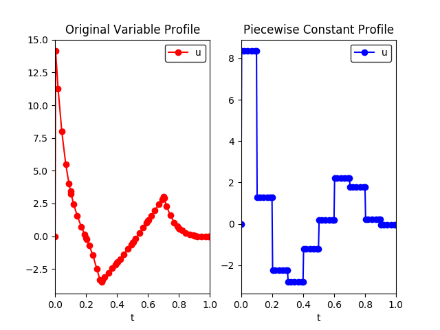
Fig. 1 (left) Profile before applying the reduce_collocation_points
function (right) Profile after applying the function, restricting
model.u to have a piecewise constant profile.
Applying Multiple Discretization Transformations
Discretizations can be applied independently to each
ContinuousSet in a model. This allows the
user great flexibility in discretizing their model. For example the same
numerical method can be applied with different resolutions:
>>> discretizer = TransformationFactory('dae.finite_difference')
>>> discretizer.apply_to(model,wrt=model.t1,nfe=10)
>>> discretizer.apply_to(model,wrt=model.t2,nfe=100)
This also allows the user to combine different methods. For example, applying
the forward difference method to one
ContinuousSet and the central finite
difference method to another
ContinuousSet:
>>> discretizer = TransformationFactory('dae.finite_difference')
>>> discretizer.apply_to(model,wrt=model.t1,scheme='FORWARD')
>>> discretizer.apply_to(model,wrt=model.t2,scheme='CENTRAL')
In addition, the user may combine finite difference and collocation discretizations. For example:
>>> disc_fe = TransformationFactory('dae.finite_difference')
>>> disc_fe.apply_to(model,wrt=model.t1,nfe=10)
>>> disc_col = TransformationFactory('dae.collocation')
>>> disc_col.apply_to(model,wrt=model.t2,nfe=10,ncp=5)
If the user would like to apply the same discretization to all
ContinuousSet components in a model, just
specify the discretization once without the ‘wrt’ keyword argument. This will
apply that scheme to all ContinuousSet
components in the model that haven’t already been discretized.
Custom Discretization Schemes
A transformation framework along with certain utility functions has been created so that advanced users may easily implement custom discretization schemes other than those listed above. The transformation framework consists of the following steps:
- Specify Discretization Options
- Discretize the ContinuousSet(s)
- Update Model Components
- Add Discretization Equations
- Return Discretized Model
If a user would like to create a custom finite difference scheme then they only have to worry about step (4) in the framework. The discretization equations for a particular scheme have been isolated from of the rest of the code for implementing the transformation. The function containing these discretization equations can be found at the top of the source code file for the transformation. For example, below is the function for the forward difference method:
def _forward_transform(v,s):
"""
Applies the Forward Difference formula of order O(h) for first derivatives
"""
    def _fwd_fun(i):
        tmp = sorted(s)
        idx = tmp.index(i)
        return 1/(tmp[idx+1]-tmp[idx])*(v(tmp[idx+1])-v(tmp[idx]))
    return _fwd_fun
In this function, ‘v’ represents the continuous variable or function that the method is being applied to. ‘s’ represents the set of discrete points in the continuous domain. In order to implement a custom finite difference method, a user would have to copy the above function and just replace the equation next to the first return statement with their method.
After implementing a custom finite difference method using the above function
template, the only other change that must be made is to add the custom method
to the ‘all_schemes’ dictionary in the dae.finite_difference
class.
In the case of a custom collocation method, changes will have to be made in steps (2) and (4) of the transformation framework. In addition to implementing the discretization equations, the user would also have to ensure that the desired collocation points are added to the ContinuousSet being discretized.
Dynamic Model Simulation
The pyomo.dae Simulator class can be used to simulate systems of ODEs and DAEs. It provides an interface to integrators available in other Python packages.
Note
The pyomo.dae Simulator does not include integrators directly. The user must have at least one of the supported Python packages installed in order to use this class.
-
class
pyomo.dae.Simulator(m, package='scipy')[source] Simulator objects allow a user to simulate a dynamic model formulated using pyomo.dae.
Parameters: - m (Pyomo Model) – The Pyomo model to be simulated should be passed as the first argument
- package (string) – The Python simulator package to use. Currently ‘scipy’ and ‘casadi’ are the only supported packages
-
get_variable_order(vartype=None)[source] This function returns the ordered list of differential variable names. The order corresponds to the order being sent to the integrator function. Knowing the order allows users to provide initial conditions for the differential equations using a list or map the profiles returned by the simulate function to the Pyomo variables.
Parameters: vartype (string or None) – Optional argument for specifying the type of variables to return the order for. The default behavior is to return the order of the differential variables. ‘time-varying’ will return the order of all the time-dependent algebraic variables identified in the model. ‘algebraic’ will return the order of algebraic variables used in the most recent call to the simulate function. ‘input’ will return the order of the time-dependent algebraic variables that were treated as inputs in the most recent call to the simulate function. Return type: list
-
initialize_model()[source] This function will initialize the model using the profile obtained from simulating the dynamic model.
-
simulate(numpoints=None, tstep=None, integrator=None, varying_inputs=None, initcon=None, integrator_options=None)[source] Simulate the model. Integrator-specific options may be specified as keyword arguments and will be passed on to the integrator.
Parameters: - numpoints (int) – The number of points for the profiles returned by the simulator. Default is 100
- tstep (int or float) – The time step to use in the profiles returned by the simulator. This is not the time step used internally by the integrators. This is an optional parameter that may be specified in place of ‘numpoints’.
- integrator (string) – The string name of the integrator to use for simulation. The default is ‘lsoda’ when using Scipy and ‘idas’ when using CasADi
- varying_inputs (
pyomo.environ.Suffix) – ASuffixobject containing the piecewise constant profiles to be used for certain time-varying algebraic variables. - initcon (list of floats) – The initial conditions for the the differential variables. This is an optional argument. If not specified then the simulator will use the current value of the differential variables at the lower bound of the ContinuousSet for the initial condition.
- integrator_options (dict) – Dictionary containing options that should be passed to the integrator. See the documentation for a specific integrator for a list of valid options.
Returns: The first return value is a 1D array of time points corresponding to the second return value which is a 2D array of the profiles for the simulated differential and algebraic variables.
Return type: numpy array, numpy array
Note
Any keyword options supported by the integrator may be specified as keyword options to the simulate function and will be passed to the integrator.
Supported Simulator Packages
The Simulator currently includes interfaces to SciPy and CasADi. ODE simulation is supported in both packages however, DAE simulation is only supported by CasADi. A list of available integrators for each package is given below. Please refer to the SciPy and CasADi documentation directly for the most up-to-date information about these packages and for more information about the various integrators and options.
- SciPy Integrators:
- ‘vode’ : Real-valued Variable-coefficient ODE solver, options for non-stiff and stiff systems
- ‘zvode’ : Complex-values Variable-coefficient ODE solver, options for non-stiff and stiff systems
- ‘lsoda’ : Real-values Variable-coefficient ODE solver, automatic switching of algorithms for non-stiff or stiff systems
- ‘dopri5’ : Explicit runge-kutta method of order (4)5 ODE solver
- ‘dop853’ : Explicit runge-kutta method of order 8(5,3) ODE solver
- CasADi Integrators:
- ‘cvodes’ : CVodes from the Sundials suite, solver for stiff or non-stiff ODE systems
- ‘idas’ : IDAS from the Sundials suite, DAE solver
- ‘collocation’ : Fixed-step implicit runge-kutta method, ODE/DAE solver
- ‘rk’ : Fixed-step explicit runge-kutta method, ODE solver
Using the Simulator
We now show how to use the Simulator to simulate the following system of ODEs:
We begin by formulating the model using pyomo.DAE
>>> m = ConcreteModel()

>>> m.t = ContinuousSet(bounds=(0.0, 10.0))

>>> m.b = Param(initialize=0.25)
>>> m.c = Param(initialize=5.0)

>>> m.omega = Var(m.t)
>>> m.theta = Var(m.t)

>>> m.domegadt = DerivativeVar(m.omega, wrt=m.t)
>>> m.dthetadt = DerivativeVar(m.theta, wrt=m.t)

Setting the initial conditions
>>> m.omega[0].fix(0.0)
>>> m.theta[0].fix(3.14 - 0.1)

>>> def _diffeq1(m, t):
...     return m.domegadt[t] == -m.b * m.omega[t] - m.c * sin(m.theta[t])
>>> m.diffeq1 = Constraint(m.t, rule=_diffeq1)

>>> def _diffeq2(m, t):
...     return m.dthetadt[t] == m.omega[t]
>>> m.diffeq2 = Constraint(m.t, rule=_diffeq2)
Notice that the initial conditions are set by fixing the values of
m.omega and m.theta at t=0 instead of being specified as extra
equality constraints. Also notice that the differential equations are
specified without using Constraint.Skip to skip enforcement at t=0. The
Simulator cannot simulate any constraints that contain if-statements in
their construction rules.
To simulate the model you must first create a Simulator object. Building this object prepares the Pyomo model for simulation with a particular Python package and performs several checks on the model to ensure compatibility with the Simulator. Be sure to read through the list of limitations at the end of this section to understand the types of models supported by the Simulator.
>>> sim = Simulator(m, package='scipy')
After creating a Simulator object, the model can be simulated by calling the
simulate function. Please see the API documentation for the
Simulator for more information about the
valid keyword arguments for this function.
>>> tsim, profiles = sim.simulate(numpoints=100, integrator='vode')
The simulate function returns numpy arrays containing time points and
the corresponding values for the dynamic variable profiles.
- Simulator Limitations:
- Differential equations must be first-order and separable
- Model can only contain a single ContinuousSet
- Can’t simulate constraints with if-statements in the construction rules
- Need to provide initial conditions for dynamic states by setting the value or using fix()
Specifying Time-Varing Inputs
The Simulator supports simulation of a system
of ODE’s or DAE’s with time-varying parameters or control inputs. Time-varying
inputs can be specified using a Pyomo Suffix. We currently only support
piecewise constant profiles. For more complex inputs defined by a continuous
function of time we recommend adding an algebraic variable and constraint to
your model.
The profile for a time-varying input should be specified
using a Python dictionary where the keys correspond to the switching times
and the values correspond to the value of the input at a time point. A
Suffix is then used to associate this dictionary with the appropriate
Var or Param and pass the information to the
Simulator. The code snippet below shows an
example.
>>> m = ConcreteModel()

>>> m.t = ContinuousSet(bounds=(0.0, 20.0))

Time-varying inputs
>>> m.b = Var(m.t)
>>> m.c = Param(m.t, default=5.0)

>>> m.omega = Var(m.t)
>>> m.theta = Var(m.t)

>>> m.domegadt = DerivativeVar(m.omega, wrt=m.t)
>>> m.dthetadt = DerivativeVar(m.theta, wrt=m.t)

Setting the initial conditions
>>> m.omega[0] = 0.0
>>> m.theta[0] = 3.14 - 0.1

>>> def _diffeq1(m, t):
...    return m.domegadt[t] == -m.b[t] * m.omega[t] - \
...                             m.c[t] * sin(m.theta[t])
>>> m.diffeq1 = Constraint(m.t, rule=_diffeq1)

>>> def _diffeq2(m, t):
...    return m.dthetadt[t] == m.omega[t]
>>> m.diffeq2 = Constraint(m.t, rule=_diffeq2)

Specifying the piecewise constant inputs
>>> b_profile = {0: 0.25, 15: 0.025}
>>> c_profile = {0: 5.0, 7: 50}

Declaring a Pyomo Suffix to pass the time-varying inputs to the Simulator
>>> m.var_input = Suffix(direction=Suffix.LOCAL)
>>> m.var_input[m.b] = b_profile
>>> m.var_input[m.c] = c_profile

Simulate the model using scipy
>>> sim = Simulator(m, package='scipy')
>>> tsim, profiles = sim.simulate(numpoints=100,
...                               integrator='vode',
...                               varying_inputs=m.var_input)
Note
The Simulator does not support multi-indexed inputs (i.e. if m.b in
the above example was indexed by another set besides m.t)
Dynamic Model Initialization
Providing a good initial guess is an important factor in solving dynamic optimization problems. There are several model initialization tools under development in pyomo.DAE to help users initialize their models. These tools will be documented here as they become available.
From Simulation
The Simulator includes a function for
initializing discretized dynamic optimization models using the profiles
returned from the simulator. An example using this function is shown below
Simulate the model using scipy
>>> sim = Simulator(m, package='scipy')
>>> tsim, profiles = sim.simulate(numpoints=100, integrator='vode',
...                               varying_inputs=m.var_input)

Discretize the model using Orthogonal Collocation
>>> discretizer = TransformationFactory('dae.collocation')
>>> discretizer.apply_to(m, nfe=10, ncp=3)

Initialize the discretized model using the simulator profiles
>>> sim.initialize_model()
Note
A model must be simulated before it can be initialized using this function