Quick Start Guide
To use Pyomo.DoE, a user must implement a subclass of the Parmest Experiment class.
The subclass must have a get_labeled_model method which returns a Pyomo ConcreteModel
containing four Pyomo Suffix components identifying the parts of the model used in
MBDoE analysis. This is in line with the convention used in the parameter estimation tool,
Parmest. The four Pyomo Suffix components are:
experiment_inputs - The experimental design decisions
experiment_outputs - The variables that are being measured
measurement_error - The error associated with the measured value of the experimental outputs. It is passed as a standard deviation or square root of the diagonal elements of the observation (measurement) error covariance matrix. Pyomo.DoE currently assumes that the observation errors are Gaussian and independent both in time and across measurements.
unknown_parameters - Those parameters in the model that are estimated from the experimental outputs
An example of the subclassed Experiment object that builds and labels the model is shown in the next few sections.
This guide illustrates the use of Pyomo.DoE using a reaction kinetics
example ([PyomoDOE-paper]).
\begin{equation}
A \xrightarrow{k_1} B \xrightarrow{k_2} C
\end{equation}
The Arrhenius equations model the temperature dependence of the reaction rate coefficients \(k_1\) and \(k_2\). Assuming a first-order reaction mechanism gives the reaction rate model shown below. Further, we assume only species A is fed to the reactor.
\begin{equation}
\begin{aligned}
k_1 & = A_1 e^{-\frac{E_1}{RT}} \\
k_2 & = A_2 e^{-\frac{E_2}{RT}} \\
\frac{d{C_A}}{dt} & = -k_1{C_A} \\
\frac{d{C_B}}{dt} & = k_1{C_A} - k_2{C_B} \\
C_{A0}& = C_A + C_B + C_C \\
C_B(t_0) & = 0 \\
C_C(t_0) & = 0 \\
\end{aligned}
\end{equation}
\(C_A(t), C_B(t), C_C(t)\) are the time-varying concentrations of the species A, B, C, respectively.
\(k_1, k_2\) are the rate constants for the two chemical reactions using an Arrhenius equation with activation energies \(E_1, E_2\) and pre-exponential factors \(A_1, A_2\).
The goal of MBDoE is to optimize the experiment design variables \(\boldsymbol{\varphi} = (C_{A0}, T(t))\), where \(C_{A0},T(t)\) are the initial concentration of species A and the time-varying reactor temperature, to maximize the precision of unknown model parameters \(\boldsymbol{\theta} = (A_1, E_1, A_2, E_2)\) by measuring \(\mathbf{y}(t)=(C_A(t), C_B(t), C_C(t))\).
The observation errors are assumed to be independent both in time and across measurements with a constant standard deviation of 1 M for each species.
Step 0: Import Pyomo and the Pyomo.DoE module and create an Experiment class
Note
This example uses the data file result.json, located in the Pyomo repository at:
pyomo/contrib/doe/examples/result.json, which contains the nominal parameter
values, and measurements for the reaction kinetics experiment.
import pyomo.environ as pyo
from pyomo.dae import ContinuousSet, DerivativeVar, Simulator
from pyomo.contrib.parmest.experiment import Experiment
Subclass the Parmest Experiment class to define the reaction
kinetics experiment and build the Pyomo ConcreteModel.
class ReactorExperiment(Experiment):
    def __init__(self, data, nfe, ncp):
        """
        Arguments
        ---------
        data: object containing vital experimental information
        nfe: number of finite elements
        ncp: number of collocation points for the finite elements
        """
        self.data = data
        self.nfe = nfe
        self.ncp = ncp
        self.model = None

        #############################
Step 1: Define the Pyomo process model
The process model for the reaction kinetics problem is shown below. Here, we build
the model without any data or discretization.
    def create_model(self):
        """
        This is an example user model provided to DoE library.
        It is a dynamic problem solved by Pyomo.DAE.

        Return
        ------
        m: a Pyomo.DAE model
        """

        m = self.model = pyo.ConcreteModel()

        # Model parameters
        m.R = pyo.Param(mutable=False, initialize=8.314)

        # Define model variables
        ########################
        # time
        m.t = ContinuousSet(bounds=[0, 1])

        # Concentrations
        m.CA = pyo.Var(m.t, within=pyo.NonNegativeReals)
        m.CB = pyo.Var(m.t, within=pyo.NonNegativeReals)
        m.CC = pyo.Var(m.t, within=pyo.NonNegativeReals)

        # Temperature
        m.T = pyo.Var(m.t, within=pyo.NonNegativeReals)

        # Arrhenius rate law equations
        m.A1 = pyo.Var(within=pyo.NonNegativeReals)
        m.E1 = pyo.Var(within=pyo.NonNegativeReals)
        m.A2 = pyo.Var(within=pyo.NonNegativeReals)
        m.E2 = pyo.Var(within=pyo.NonNegativeReals)

        # Differential variables (Conc.)
        m.dCAdt = DerivativeVar(m.CA, wrt=m.t)
        m.dCBdt = DerivativeVar(m.CB, wrt=m.t)

        ########################
        # End variable def.

        # Equation definition
        ########################

        # Expression for rate constants
        @m.Expression(m.t)
        def k1(m, t):
            return m.A1 * pyo.exp(-m.E1 * 1000 / (m.R * m.T[t]))

        @m.Expression(m.t)
        def k2(m, t):
            return m.A2 * pyo.exp(-m.E2 * 1000 / (m.R * m.T[t]))

        # Concentration odes
        @m.Constraint(m.t)
        def CA_rxn_ode(m, t):
            return m.dCAdt[t] == -m.k1[t] * m.CA[t]

        @m.Constraint(m.t)
        def CB_rxn_ode(m, t):
            return m.dCBdt[t] == m.k1[t] * m.CA[t] - m.k2[t] * m.CB[t]

        # algebraic balance for concentration of C
        # Valid because the reaction system (A --> B --> C) is equimolar
        @m.Constraint(m.t)
        def CC_balance(m, t):
            return m.CA[0] == m.CA[t] + m.CB[t] + m.CC[t]

        ########################
Step 2: Finalize the Pyomo process model
Here, we add data to the model and discretize it. This step is required before
the model can be labeled.
    def finalize_model(self):
        """
        Example finalize model function. There are two main tasks
        here:

            1. Extracting useful information for the model to align
               with the experiment. (Here: CA0, t_final, t_control)
            2. Discretizing the model subject to this information.

        """
        m = self.model

        # Unpacking data before simulation
        control_points = self.data["control_points"]

        # Set initial concentration values for the experiment
        m.CA[0].value = self.data["CA0"]
        m.CB[0].fix(self.data["CB0"])

        # Update model time `t` with time range and control time points
        m.t.update(self.data["t_range"])
        m.t.update(control_points)

        # Fix the unknown parameter values
        m.A1.fix(self.data["A1"])
        m.A2.fix(self.data["A2"])
        m.E1.fix(self.data["E1"])
        m.E2.fix(self.data["E2"])

        # Add upper and lower bounds to the design variable, CA[0]
        m.CA[0].setlb(self.data["CA_bounds"][0])
        m.CA[0].setub(self.data["CA_bounds"][1])

        m.t_control = control_points

        # Discretizing the model
        discr = pyo.TransformationFactory("dae.collocation")
        discr.apply_to(m, nfe=self.nfe, ncp=self.ncp, wrt=m.t)

        # Initializing Temperature in the model
        cv = None
        for t in m.t:
            if t in control_points:
                cv = control_points[t]
                m.T[t].fix()
            m.T[t].setlb(self.data["T_bounds"][0])
            m.T[t].setub(self.data["T_bounds"][1])
            m.T[t] = cv

        # Make a constraint that holds temperature constant between control time points
        @m.Constraint(m.t - control_points)
        def T_control(m, t):
            """
            Piecewise constant temperature between control points
            """
            neighbour_t = max(tc for tc in control_points if tc < t)
            return m.T[t] == m.T[neighbour_t]

        #########################
Step 4: Implement the get_labeled_model method
This method utilizes the previous 3 steps and is used by Pyomo.DoE to build the model
to perform optimal experimental design.
    def get_labeled_model(self):
        if self.model is None:
            self.create_model()
            self.finalize_model()
            self.label_experiment()
        return self.model
Step 5: Exploratory analysis (Enumeration)
After creating the subclass of the Experiment class, exploratory analysis is
suggested to systematically enumerate the experimental design space and identify regions
that provide high information content about the model parameters, as quantified by
the A-, D-, E-, and ME-optimality criteria.
Additionally, it helps to initialize the model for the optimal experimental design step.
Pyomo.DoE can perform exploratory sensitivity analysis with the compute_FIM_full_factorial() method.
The compute_FIM_full_factorial() method generates a grid over the design space as specified by the user.
Each grid point represents an MBDoE problem solved using the compute_FIM() method.
In this way, sensitivity of the FIM over the design space can be evaluated.
Pyomo.DoE supports plotting the results from the compute_FIM_full_factorial() method
with the draw_factorial_figure() method.
The following code defines the run_reactor_doe function. This function encapsulates
the workflow for both sensitivity analysis (Step 5) and optimal design (Step 6).
from pyomo.common.dependencies import numpy as np, pathlib

from pyomo.contrib.doe.examples.reactor_experiment import ReactorExperiment
from pyomo.contrib.doe import DesignOfExperiments

import pyomo.environ as pyo

import json


# Example for sensitivity analysis on the reactor experiment
# After sensitivity analysis is done, we perform optimal DoE
def run_reactor_doe(
    n_points_for_C0: int = 9,
    n_points_for_T0: int = 9,
    C0_bounds_for_factorial: tuple = (1, 5),
    T0_bounds_for_factorial: tuple = (300, 700),
    compute_FIM_full_factorial=True,
    plot_factorial_results=True,
    figure_file_name="example_reactor_compute_FIM",
    log_scale=False,
    run_optimal_doe=True,
):
    """
    This function demonstrates how to perform sensitivity analysis on the reactor

    Parameters
    ----------
    n_points_for_C0 : int, optional
        number of points to use for the C0 design range, by default 9
    n_points_for_T0 : int, optional
        number of points to use for the T0 design range, by default 9
    compute_FIM_full_factorial : bool, optional
        whether to compute the full factorial design, by default True
    plot_factorial_results : bool, optional
        whether to plot the results of the full factorial design, by default True
    figure_file_name : str, optional
        file name to save the factorial figure, by default "example_reactor_compute_FIM"
    run_optimal_doe : bool, optional
        whether to run the optimal DoE, by default True
    """
    # Read in file
    DATA_DIR = pathlib.Path(__file__).parent
    file_path = DATA_DIR / "result.json"

    with open(file_path) as f:
        data_ex = json.load(f)

    # Put temperature control time points into correct format for reactor experiment
    data_ex["control_points"] = {
        float(k): v for k, v in data_ex["control_points"].items()
    }

    # Create a ReactorExperiment object; data and discretization information are part
    # of the constructor of this object
    experiment = ReactorExperiment(data=data_ex, nfe=10, ncp=3)

    # Use a central difference, with step size 1e-3
    fd_formula = "central"
    step_size = 1e-3

    # Use the determinant objective with scaled sensitivity matrix
    objective_option = "determinant"
    scale_nominal_param_value = True

    # Create the DesignOfExperiments object
    # We will not be passing any prior information in this example
    # and allow the experiment object and the DesignOfExperiments
    # call of ``run_doe`` perform model initialization.
    doe_obj = DesignOfExperiments(
        experiment,
        fd_formula=fd_formula,
        step=step_size,
        objective_option=objective_option,
        scale_constant_value=1,
        scale_nominal_param_value=scale_nominal_param_value,
        prior_FIM=None,
        jac_initial=None,
        fim_initial=None,
        L_diagonal_lower_bound=1e-7,
        solver=None,
        tee=False,
        get_labeled_model_args=None,
        _Cholesky_option=True,
        _only_compute_fim_lower=True,
    )
    if compute_FIM_full_factorial:
        # Make design ranges to compute the full factorial design
        design_ranges = {
            "CA[0]": [*C0_bounds_for_factorial, n_points_for_C0],
            "T[0]": [*T0_bounds_for_factorial, n_points_for_T0],
        }

        # Compute the full factorial design with the sequential FIM calculation
        doe_obj.compute_FIM_full_factorial(
            design_ranges=design_ranges, method="sequential"
        )
    if plot_factorial_results:
        # Plot the results
        doe_obj.draw_factorial_figure(
            sensitivity_design_variables=["CA[0]", "T[0]"],
            fixed_design_variables={
                "T[0.125]": 300,
                "T[0.25]": 300,
                "T[0.375]": 300,
                "T[0.5]": 300,
                "T[0.625]": 300,
                "T[0.75]": 300,
                "T[0.875]": 300,
                "T[1]": 300,
            },
            title_text="Reactor Example",
            xlabel_text="Concentration of A (M)",
            ylabel_text="Initial Temperature (K)",
            figure_file_name=figure_file_name,
            log_scale=log_scale,
        )

    ###########################
    # End sensitivity analysis

    # Begin optimal DoE
    ####################
    if run_optimal_doe:
        doe_obj.run_doe()

        # Print out a results summary
        print("Optimal experiment values: ")
        print(
            "\tInitial concentration: {:.2f}".format(
                doe_obj.results["Experiment Design"][0]
            )
        )
        print(
            ("\tTemperature values: [" + "{:.2f}, " * 8 + "{:.2f}]").format(
                *doe_obj.results["Experiment Design"][1:]
            )
        )
        print("FIM at optimal design:\n {}".format(np.array(doe_obj.results["FIM"])))
        print(
            "Objective value at optimal design: {:.2f}".format(
                pyo.value(doe_obj.model.objective)
            )
        )

        print(doe_obj.results["Experiment Design Names"])

        ###################
        # End optimal DoE

    return doe_obj
After defining the function, we will call it to perform the exploratory analysis and
the optimal experimental design.
run_reactor_doe(figure_file_name=None)
A design exploration for the initial concentration and temperature as experimental
design variables with 9 values for each, produces the the five figures for
five optimality criteria using the compute_FIM_full_factorial and
draw_factorial_figure methods as shown below:
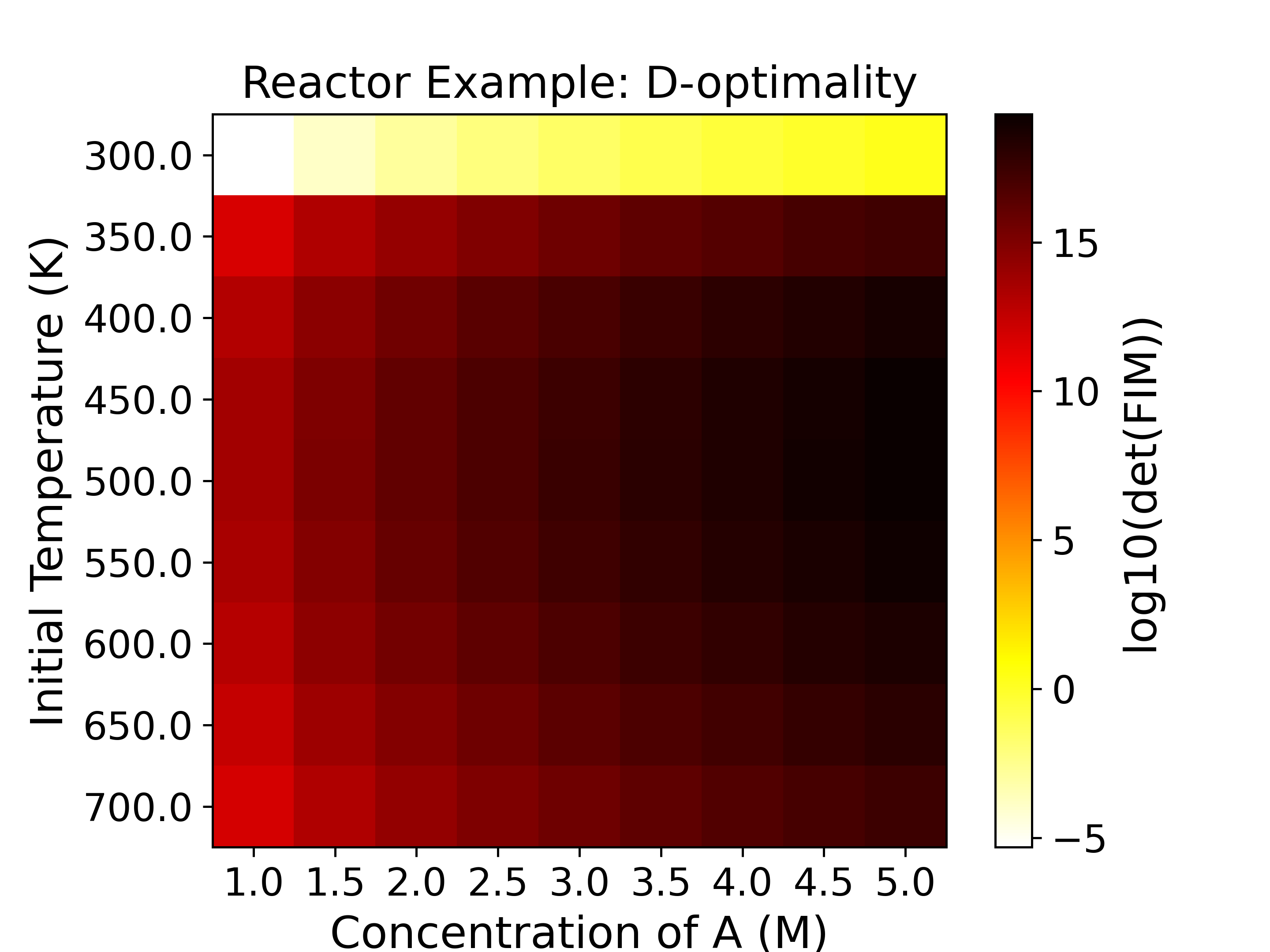
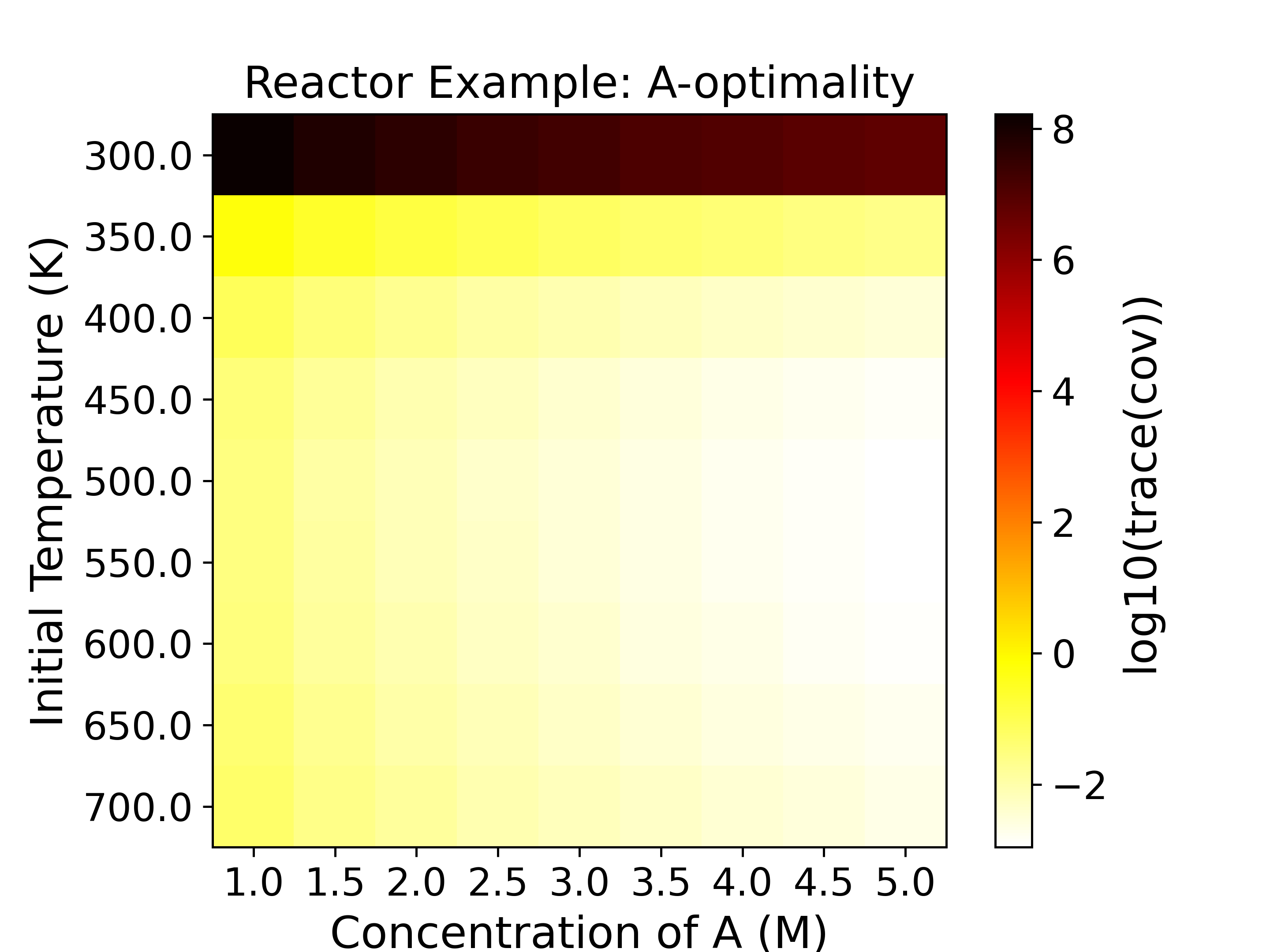
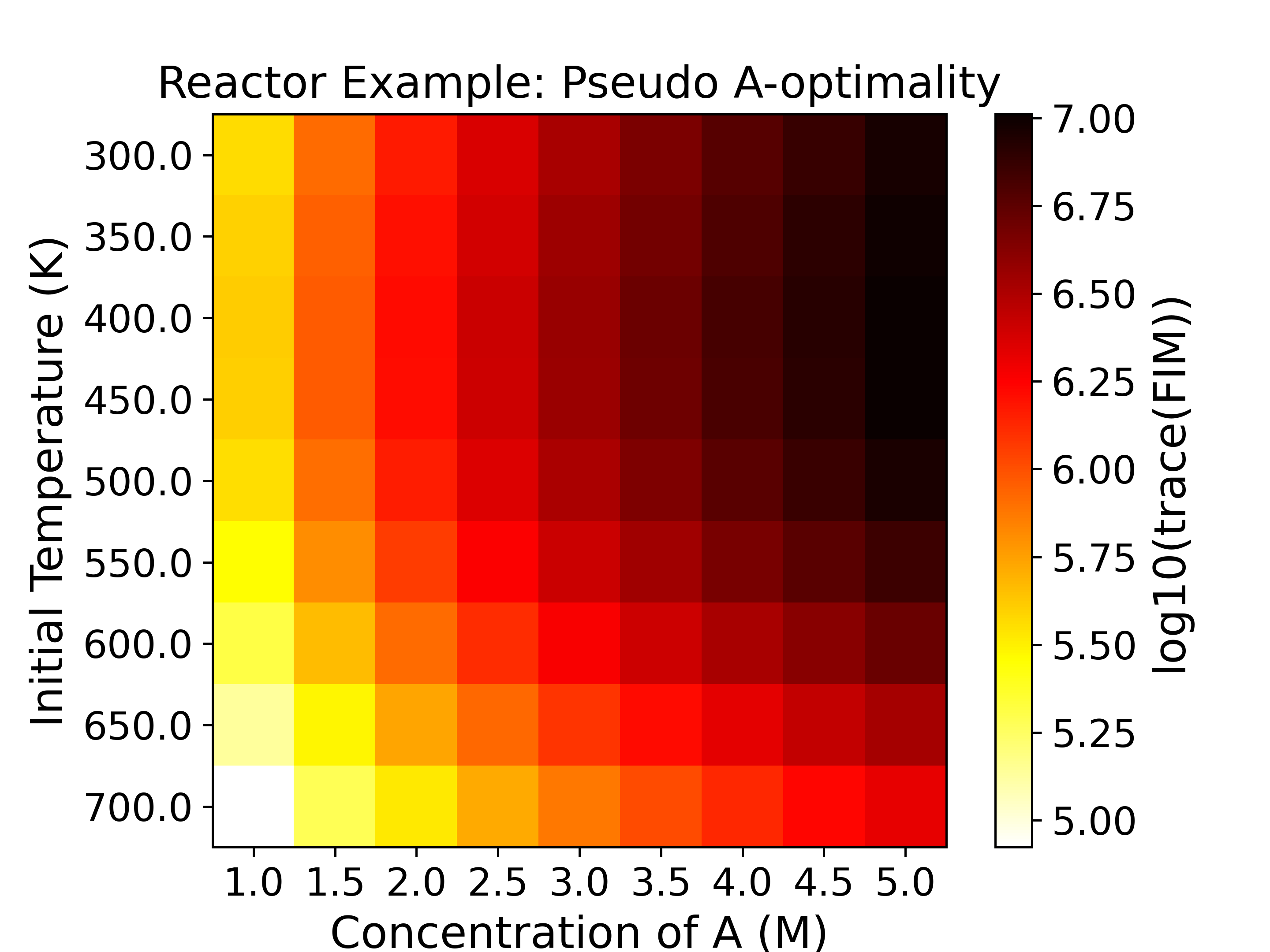
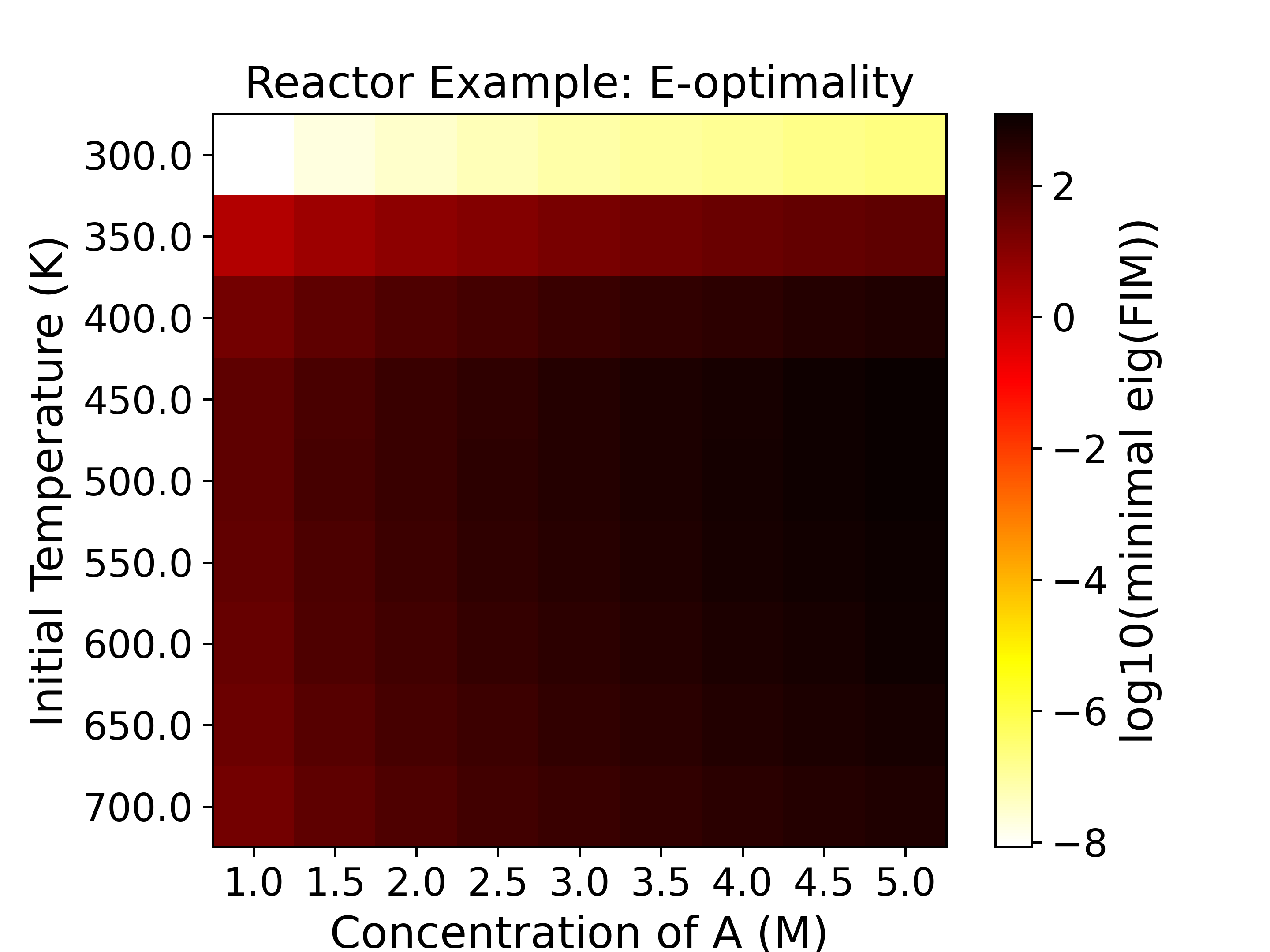
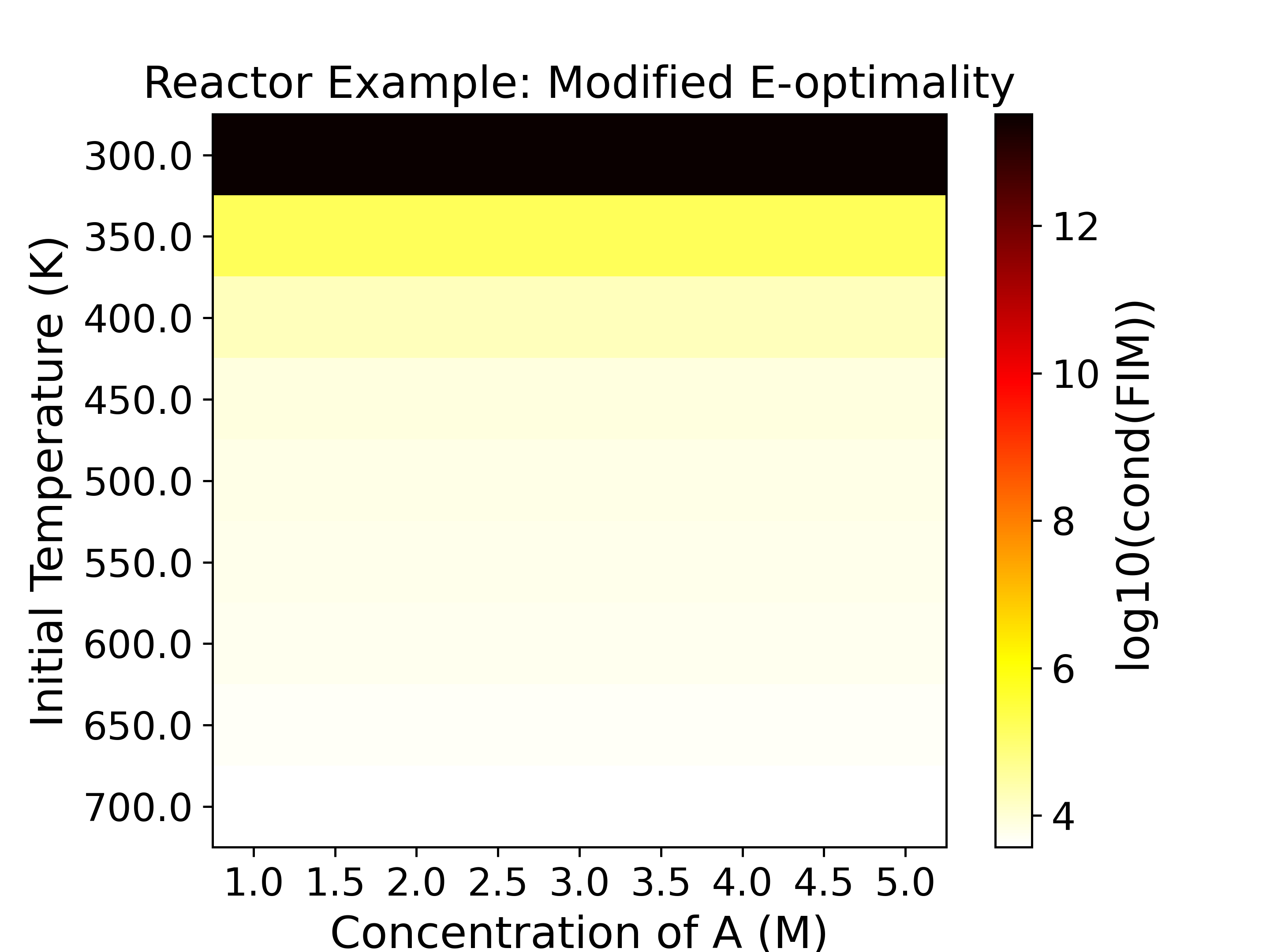
The heatmaps show the variation of a FIM-based objective function
(specified by the user) over a grid of the experimental design space.
Therefore, the heatmaps are a representation of the experimental
information of various design conditions. Horizontal and vertical axes
are the two experimental design variables, while the color of each
grid shows the experimental information content. For example,
the D-optimality (upper left subplot) heatmap figure shows that the
most informative region is around \(C_{A0}=5.0\) M, \(T=500.0\) K with
a \(\log_{10}\) determinant of FIM being around 19,
while the least informative region is around \(C_{A0}=1.0\) M, \(T=300.0\) K,
with a \(\log_{10}\) determinant of FIM being around -5. For D-, Pseudo A-, and
E-optimality we want to maximize the objective function, while for A- and Modified
E-optimality we want to minimize the objective function.
In this sensitivity analysis plot (heatmap), we only varied the initial
concentration and the initial temperature, while the temperature at other time
points is fixed at 300 K.
\[
T(t) = \begin{cases}
T_0, & t \le 0.125 \\
300\ \text{K}, & t > 0.125
\end{cases}
\]
If \(T_0 = 300\ \text{K}\), the reaction is conducted under strictly isothermal
conditions. Because the temperature is constant, the sensitivities of the species
concentrations with respect to the Arrhenius parameters (\(A_i\) and \(E_i\))
become linearly dependent. This high correlation means the effects of the
pre-exponential factor and the activation energy cannot be uniquely distinguished
from the measurements. Consequently, the Fisher Information Matrix (FIM) becomes
ill-conditioned, resulting in a near-zero determinant and a very large condition number.
To break this correlation and make the parameters identifiable, introducing a time-
varying temperature profile (for example, a temperature step or a ramp) is required.
As shown in the heatmap, when the initial temperature \(T_0\) differs from the
subsequent 300 K baseline, such a temperature change breaks the linear dependence,
yielding a well-conditioned FIM and identifiable parameters.